Multi-horizon Forecasting using Temporal Fusion Transformers – A Comprehensive Overview – Part 2
By Dvir Ben Or and Michael Kolomenkin
This post is a continuation of the first post on Multi-horizon Forecasting (MHF). The first post described challenges associated with MHF, the scenarios where MHF is beneficial, and the advantages of using a Temporal Fusion Transformer (TFT) for MHF. It also formally defined the optimization task used for training the TFT. This post provides a detailed overview of the structure of the TFT model and demonstrates how the model’s outputs can be used for further analysis and inspection. These explanations are accompanied by code examples.
The code is also available as part of the tft-torch package, which implements the TFT using PyTorch framework.
The TFT model was originally presented in the paper “Temporal Fusion Transformers for Interpretable Multi-horizon Time Series Forecasting”1, written by Bryan Lim, Sercan O. Arik, Nicolas Loeff, and Tomas Pfister (from Oxford University and Google Cloud).
Model Structure
At first glance, the model’s diagram might seem a bit intimidating, but we’ll try to clarify it as much as possible.
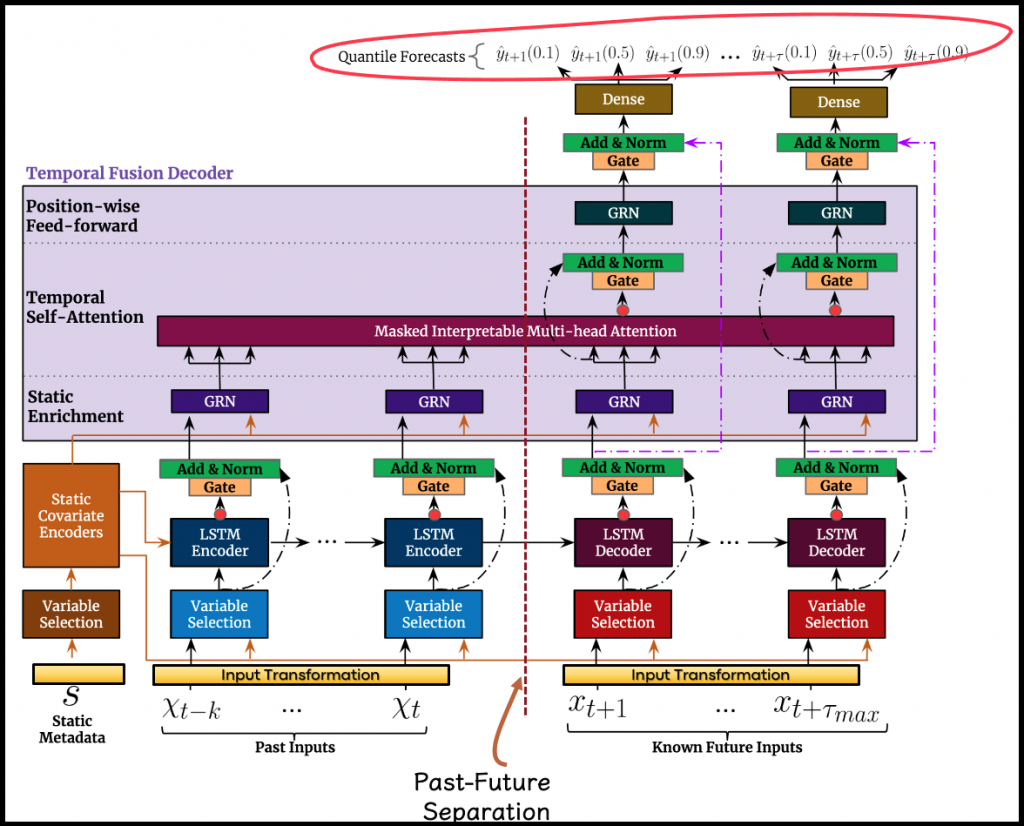
At the bottom of the diagram, we see where the three input types are fed into the model; the static attributes, the historical time-series, and the known future inputs. Note the virtual dashed line, which “separates” historical and future information.
At the top of the diagram, the quantile estimation outputs (circled in red) are generated for each future step. According to these outputs, the loss, described in the first post, is computed.
Input Transformation
Every information channel flowing into the model has a separate, dedicated, learned transformation, which is applied to the input variables composing it. These transformations are used to transform each input variable into a (\(d_{model}\))-dimensional vector, corresponding to the dimensions of subsequent layers, to allow skip-connections. In the case of the temporal channels (historical / future time-series), these learned transformations are shared across time, thus, they act similarly on each time step.
Each information channel can be composed of numerical and categorical attributes.
- The input transformation applied to the categorical variables includes embedding layers that map each categorical entity to a corresponding vector representation (as is usually performed in recommender systems or word embeddings, in natural language processing).
- The numerical variables go through dedicated linear layers, where each variable has a separate linear layer.
Eventually, each input variable is mapped into a vector of length \(d_{model}\). The hyper-parameter \(d_{model}\) is one of the few hyper-parameters that control the model’s structure and composition.
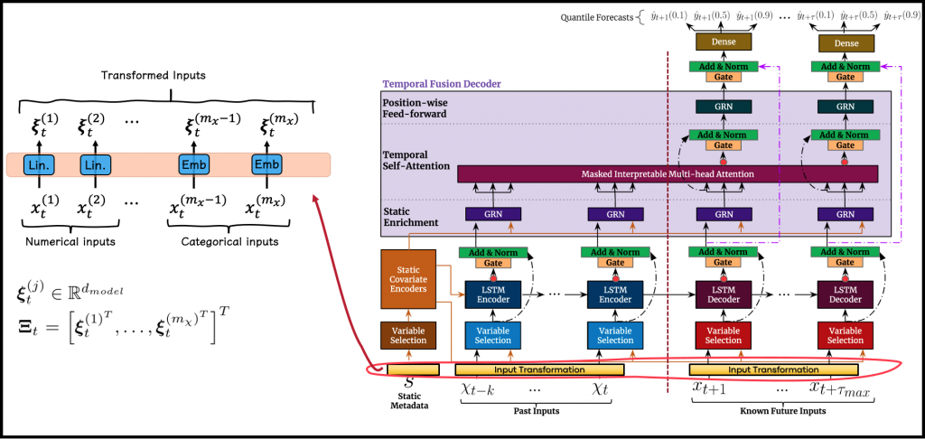
The illustrated example to the left of Figure 2 describes a temporal input channel at a specific time-step, but it behaves similarly on the static inputs as well. As depicted in the figure, we use \(\boldsymbol{\xi}^{(j)}_{t}\) to denote the resulting signal after processing the \(j\)-th input variable at the \(t\)-th time step with the corresponding learned transformation (subscript \(t\) is irrelevant for static inputs). As mentioned, each of these \(\boldsymbol{\xi}^{(j)}_{t}\), is of \(d_{model}\) dimension. We also use \(\boldsymbol{\Xi}_{t}\) to denote the flattened concatenation of the transformed inputs in a specific input channel, for a specific time-step.
The following snippet suggests a possible implementation of the input transformation phase, which is available as part of tft-torch:
from torch import nn

class NumericInputTransformation(nn.Module):
    """
    A module for transforming/embeddings the set of numeric input variables from a single input channel.
    Each input variable will be projected using a dedicated linear layer to a vector with width state_size.
    The result of applying this module is a list, with length num_inputs, that contains the embedding of each input
    variable for all the observations and time steps.

    Parameters
    ----------
    num_inputs : int
        The quantity of numeric input variables associated with this module.
    state_size : int
        The state size of the model, which determines the embedding dimension/width.
    """

    def __init__(self, num_inputs: int, state_size: int):
        super(NumericInputTransformation, self).__init__()
        self.num_inputs = num_inputs
        self.state_size = state_size

        self.numeric_projection_layers = nn.ModuleList()
        for _ in range(self.num_inputs):
            self.numeric_projection_layers.append(nn.Linear(1, self.state_size))

    def forward(self, x: torch.tensor) -> List[torch.tensor]:
        # every input variable is projected using its dedicated linear layer,
        # the results are stored as a list
        projections = []
        for i in range(self.num_inputs):
            projections.append(self.numeric_projection_layers[i](x[:, [i]]))

        return projections


class CategoricalInputTransformation(nn.Module):
    """
    A module for transforming/embeddings the set of categorical input variables from a single input channel.
    Each input variable will be projected using a dedicated embedding layer to a vector with width state_size.
    The result of applying this module is a list, with length num_inputs, that contains the embedding of each input
    variable for all the observations and time steps.

    Parameters
    ----------
    num_inputs : int
        The quantity of categorical input variables associated with this module.
    state_size : int
        The state size of the model, which determines the embedding dimension/width.
    cardinalities: List[int]
        The quantity of categories associated with each of the input variables.
    """

    def __init__(self, num_inputs: int, state_size: int, cardinalities: List[int]):
        super(CategoricalInputTransformation, self).__init__()
        self.num_inputs = num_inputs
        self.state_size = state_size
        self.cardinalities = cardinalities

        # layers for processing the categorical inputs
        self.categorical_embedding_layers = nn.ModuleList()
        for idx, cardinality in enumerate(self.cardinalities):
            self.categorical_embedding_layers.append(nn.Embedding(cardinality, self.state_size))

    def forward(self, x: torch.tensor) -> List[torch.tensor]:
        # every input variable is projected using its dedicated embedding layer,
        # the results are stored as a list
        embeddings = []
        for i in range(self.num_inputs):
            embeddings.append(self.categorical_embedding_layers[i](x[:, i]))

        return embeddings


class InputChannelEmbedding(nn.Module):
    """
    A module to handle the transformation/embedding of an input channel composed of numeric tensors and categorical
    tensors.
    It holds a NumericInputTransformation module for handling the embedding of the numeric inputs,
    and a CategoricalInputTransformation module for handling the embedding of the categorical inputs.

    Parameters
    ----------
    state_size : int
        The state size of the model, which determines the embedding dimension/width of each input variable.
    num_numeric : int
        The quantity of numeric input variables associated with the input channel.
    num_categorical : int
        The quantity of categorical input variables associated with the input channel.
    categorical_cardinalities: List[int]
        The quantity of categories associated with each of the categorical input variables.
    time_distribute: Optional[bool]
        A boolean indicating whether to wrap the composing transformations using the ``TimeDistributed`` module.
    """

    def __init__(self, state_size: int, num_numeric: int, num_categorical: int, categorical_cardinalities: List[int],
                 time_distribute: Optional[bool] = False):
        super(InputChannelEmbedding, self).__init__()

        self.state_size = state_size
        self.num_numeric = num_numeric
        self.num_categorical = num_categorical
        self.categorical_cardinalities = categorical_cardinalities
        self.time_distribute = time_distribute

        if self.time_distribute:
            self.numeric_transform = TimeDistributed(
                NumericInputTransformation(num_inputs=num_numeric, state_size=state_size), return_reshaped=False)
            self.categorical_transform = TimeDistributed(
                CategoricalInputTransformation(num_inputs=num_categorical, state_size=state_size,
                                               cardinalities=categorical_cardinalities), return_reshaped=False)
        else:
            self.numeric_transform = NumericInputTransformation(num_inputs=num_numeric, state_size=state_size)
            self.categorical_transform = CategoricalInputTransformation(num_inputs=num_categorical,
                                                                        state_size=state_size,
                                                                        cardinalities=categorical_cardinalities)

    def forward(self, x_numeric, x_categorical) -> torch.tensor:
        batch_shape = x_numeric.shape

        processed_numeric = self.numeric_transform(x_numeric)
        processed_categorical = self.categorical_transform(x_categorical)
        # Both of the returned values, "processed_numeric" and "processed_categorical" are lists,
        # with "num_numeric" elements and "num_categorical" respectively - each element in these lists corresponds
        # to a single input variable, and is represent by its embedding, shaped as:
        # [(num_samples * num_temporal_steps) x state_size]
        # (for the static input channel, num_temporal_steps is irrelevant and can be treated as 1

        # the resulting embeddings for all the input varaibles are concatenated to a flattened representation
        merged_transformations = torch.cat(processed_numeric + processed_categorical, dim=1)
        # Dimensions:
        # merged_transformations: [(num_samples * num_temporal_steps) x (state_size * total_input_variables)]
        # total_input_variables stands for the amount of all input variables in the specific input channel, i.e
        # num_numeric + num_categorical

        # for temporal data we return the resulting tensor to its 3-dimensional shape
        if self.time_distribute:
            merged_transformations = merged_transformations.view(batch_shape[0], batch_shape[1], -1)
            # In that case:
            # merged_transformations: [num_samples x num_temporal_steps x (state_size * total_input_variables)]

        return merged_transformations
Note that the InputChannelEmbedding module employs a module named TimeDistributed , which is used for wrapping a given module and applying it to a tensor representing a sequence as follows:
class TimeDistributed(nn.Module):
    """
    This module can wrap any given module and stacks the time dimension with the batch dimension of the inputs
    before applying the module.
    Borrowed from this fruitful `discussion thread
    <https://discuss.pytorch.org/t/any-pytorch-function-can-work-as-keras-timedistributed/1346/4>`_.

    Parameters
    ----------
    module : nn.Module
        The wrapped module.
    batch_first: bool
        A boolean indicating whether the batch dimension is expected to be the first dimension of the input or not.
    return_reshaped: bool
        A boolean indicating whether to return the output in the corresponding original shape or not.
    """

    def __init__(self, module: nn.Module, batch_first: bool = True, return_reshaped: bool = True):
        super(TimeDistributed, self).__init__()
        self.module: nn.Module = module  # the wrapped module
        self.batch_first: bool = batch_first  # indicates the dimensions order of the sequential data.
        self.return_reshaped: bool = return_reshaped

    def forward(self, x):

        # in case the incoming tensor is a two-dimensional tensor - infer no temporal information is involved,
        # and simply apply the module
        if len(x.size()) <= 2:
            return self.module(x)

        # Squash samples and time-steps into a single axis
        x_reshape = x.contiguous().view(-1, x.size(-1))  # (samples * time-steps, input_size)
        # apply the module on each time-step separately
        y = self.module(x_reshape)

        # reshaping the module output as sequential tensor (if required)
        if self.return_reshaped:
            if self.batch_first:
                y = y.contiguous().view(x.size(0), -1, y.size(-1))  # (samples, time-steps, output_size)
            else:
                y = y.view(-1, x.size(1), y.size(-1))  # (time-steps, samples, output_size)

        return y
Gating Mechanism
As evidenced by the diagram above, there are certain architecture blocks that are repeatedly used across the model. In practice, a modularization of this kind facilitates the implementation of such a model.
One such block is the GatedResidualNetwork (GRN). GRN increases the model’s flexibility. It allows controlling the degree of non-linear processing of the input. The required degree is hard to set in advance. For example, noisy inputs benefit from simpler processing. GRN provides the ability to apply non-linear processing only when it is required.
GRN achieves flexibility by using a gating mechanism. Gating is the process that allows the model to skip some connections, attenuate some of the inputs, or replace them with an identity transformation. In doing so, the model adapts the effective depth and complexity of the network to meet its needs.
Figure 3 Illustrates the GRN’s operations. Its ability to effectively skip unnecessary processing is achieved thanks to the following:
- A residual connection to the primary input of the block. The connection is depicted by the dotted line, traced from the input \(a\) to the normalization block.
- A block named GatedLinearUnit (GLU), which controls the degree to which the GRN contributes to the original input of the block, denoted as \(a\). The GLU promotes flexibility by possibly attenuating the processed inputs, using a sigmoid function.
- The output of the GRN is the sum of the original input and the output of the GLU. Thus, if the output of the GLU is zero, the GRN serves as an identity function.
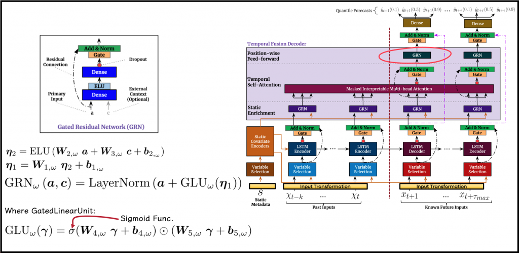
As depicted in the diagram, every GRN is fed with a primary input, \(\boldsymbol{a}\), and optionally with the context input, denoted as \(\boldsymbol{c}\). The GRN acts as follows:
- In cases where the context input, \(\boldsymbol{c}\), is irrelevant, it can be treated as zero in the equations.
- \(ELU()\), which stands for Exponential Linear Unit, is an activation function, responsible for non-linearity.
- After applying the parametrized and learned projections, represented by \(\boldsymbol{W}_{i,\omega}\) and \(\boldsymbol{b}_{i,\omega}\), the resulting tensors \(\boldsymbol{\eta}_1\) and \(\boldsymbol{\eta}_2\) are of size \(d_{model}\).
- The Layer Normalization step is a normalization operating at the level of a single observation, thus overcoming the shortcomings of Batch Normalization layers. This paper explains how layer normalization overcomes the drawbacks of batch normalization.
- Absent in the equations, as it is exclusively relevant for training, a Dropout mechanism is applied prior to the gating operation.
A possible implementation of GRN and GLU is as follows:
class GatedLinearUnit(nn.Module):
    """
    This module is also known as  **GLU** - Formulated in:
    `Dauphin, Yann N., et al. "Language modeling with gated convolutional networks."
    International conference on machine learning. PMLR, 2017
    <https://arxiv.org/abs/1612.08083>`_.

    The output of the layer is a linear projection (X * W + b) modulated by the gates **sigmoid** (X * V + c).
    These gates multiply each element of the matrix X * W + b and control the information passed on in the hierarchy.
    This unit is a simplified gating mechanism for non-deterministic gates that reduce the vanishing gradient problem,
    by having linear units coupled to the gates. This retains the non-linear capabilities of the layer while allowing
    the gradient to propagate through the linear unit without scaling.

    Parameters
    ----------
    input_dim: int
        The embedding size of the input.
    """

    def __init__(self, input_dim: int):
        super(GatedLinearUnit, self).__init__()

        # Two dimension-preserving dense layers
        self.fc1 = nn.Linear(input_dim, input_dim)
        self.fc2 = nn.Linear(input_dim, input_dim)
        self.sigmoid = nn.Sigmoid()

    def forward(self, x):
        sig = self.sigmoid(self.fc1(x))
        x = self.fc2(x)
        return torch.mul(sig, x)


class GatedResidualNetwork(nn.Module):
    """
    This module, known as **GRN**, takes in a primary input (x) and an optional context vector (c).
    It uses a ``GatedLinearUnit`` for controlling the extent to which the module will contribute to the original input
    (x), potentially skipping over the layer entirely as the GLU outputs could be all close to zero, by that suppressing
    the non-linear contribution.
    In cases where no context vector is used, the GRN simply treats the context input as zero.
    During training, dropout is applied before the gating layer.

    Parameters
    ----------
    input_dim: int
        The embedding width/dimension of the input.
    hidden_dim: int
        The intermediate embedding width.
    output_dim: int
        The embedding width of the output tensors.
    dropout: Optional[float]
        The dropout rate associated with the component.
    context_dim: Optional[int]
        The embedding width of the context signal expected to be fed as an auxiliary input to this component.
    batch_first: Optional[bool]
        A boolean indicating whether the batch dimension is expected to be the first dimension of the input or not.
    """

    def __init__(self, input_dim: int, hidden_dim: int, output_dim: int,
                 dropout: Optional[float] = 0.05,
                 context_dim: Optional[int] = None,
                 batch_first: Optional[bool] = True):
        super(GatedResidualNetwork, self).__init__()
        self.input_dim = input_dim
        self.output_dim = output_dim
        self.context_dim = context_dim
        self.hidden_dim = hidden_dim
        self.dropout = dropout

        # =================================================
        # Input conditioning components (Eq.4 in the original paper)
        # =================================================
        # for using direct residual connection the dimension of the input must match the output dimension.
        # otherwise, we'll need to project the input for creating this residual connection
        self.project_residual: bool = self.input_dim != self.output_dim
        if self.project_residual:
            self.skip_layer = TimeDistributed(nn.Linear(self.input_dim, self.output_dim))

        # A linear layer for projecting the primary input (acts across time if necessary)
        self.fc1 = TimeDistributed(nn.Linear(self.input_dim, self.hidden_dim), batch_first=batch_first)

        # In case we expect context input, an additional linear layer will project the context
        if self.context_dim is not None:
            self.context_projection = TimeDistributed(nn.Linear(self.context_dim, self.hidden_dim, bias=False),
                                                      batch_first=batch_first)
        # non-linearity to be applied on the sum of the projections
        self.elu1 = nn.ELU()

        # ============================================================
        # Further projection components (Eq.3 in the original paper)
        # ============================================================
        # additional projection on top of the non-linearity
        self.fc2 = TimeDistributed(nn.Linear(self.hidden_dim, self.output_dim), batch_first=batch_first)

        # ============================================================
        # Output gating components (Eq.2 in the original paper)
        # ============================================================
        self.dropout = nn.Dropout(self.dropout)
        self.gate = TimeDistributed(GatedLinearUnit(self.output_dim), batch_first=batch_first)
        self.layernorm = TimeDistributed(nn.LayerNorm(self.output_dim), batch_first=batch_first)

    def forward(self, x, context=None):

        # compute residual (for skipping) if necessary
        if self.project_residual:
            residual = self.skip_layer(x)
        else:
            residual = x
        # ===========================
        # Compute Eq.4
        # ===========================
        x = self.fc1(x)
        if context is not None:
            context = self.context_projection(context)
            x = x + context

        # compute eta_2 (according to paper)
        x = self.elu1(x)

        # ===========================
        # Compute Eq.3
        # ===========================
        # compute eta_1 (according to paper)
        x = self.fc2(x)

        # ===========================
        # Compute Eq.2
        # ===========================
        x = self.dropout(x)
        x = self.gate(x)
        # perform skipping using the residual
        x = x + residual
        # apply normalization layer
        x = self.layernorm(x)

        return x
Note that, in other stages of the model flow, gating and residual connections coming from earlier processing phases are used, including those found outside the context of a GRN. This composite operation can be termed GateAddNorm, and its implementation is as follows:
class GateAddNorm(nn.Module):
    """
    This module encapsulates an operation performed multiple times across the TemporalFusionTransformer model.
    The composite operation includes:
    a. A *Dropout* layer.
    b. Gating using a ``GatedLinearUnit``.
    c. A residual connection to an "earlier" signal from the forward pass of the parent model.
    d. Layer normalization.

    Parameters
    ----------
    input_dim: int
        The dimension associated with the expected input of this module.
    dropout: Optional[float]
        The dropout rate associated with the component.
    """

    def __init__(self, input_dim: int, dropout: Optional[float] = None):
        super(GateAddNorm, self).__init__()
        self.dropout_rate = dropout
        if dropout:
            self.dropout_layer = nn.Dropout(self.dropout_rate)
        self.gate = TimeDistributed(GatedLinearUnit(input_dim), batch_first=True)
        self.layernorm = TimeDistributed(nn.LayerNorm(input_dim), batch_first=True)

    def forward(self, x, residual=None):
        if self.dropout_rate:
            x = self.dropout_layer(x)
        x = self.gate(x)
        # perform skipping
        if residual is not None:
            x = x + residual
        # apply normalization layer
        x = self.layernorm(x)

        return x
Variable Selection
The target signal we wish to predict might be unrelated to some of the input variables. Moreover, the input variables’ relevance to the target signal is unknown in advance and, therefore, should be learned. For that reason, the authors designed a block to handle the soft-selection of variables. This block is termed VariableSelectionNetwork (VSN).
The VSN block follows the input transformation block, and like the input transformation block, the VSN block is applied similarly, but separately, to the static inputs and the temporal inputs. Note that the different colors in the diagram (Figure 4) indicate separate VSN blocks for each information channel. As before, for the temporal channels, the block is shared across time (using the TimeDistributed module).
The VSN blocks provide insights regarding which inputs are more important or significant to the prediction task (as we’ll soon see, this is one of the explainable outputs we can retrieve from the model). In addition, this component removes noisy inputs, or inputs that do not contribute to the prediction task and might harm the model’s performance. The VSN improves the model’s performance by allowing the model to focus its capacity on processing significant attributes.
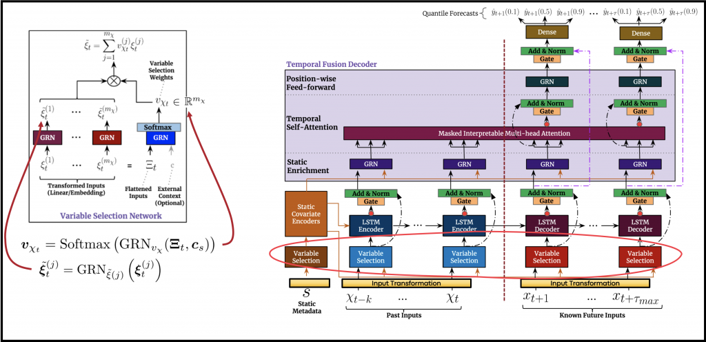
VSN is applied right after the input transformation. Every transformed input, \(\boldsymbol{\xi}^{(j)}_{t}\), is processed by a separate GRN (shared across time, but acting separately for each time-step), responsible for non-linear processing, resulting in \(\boldsymbol{\tilde{\xi}}^{(j)}_{t}\).
A separate GRN is also dedicated to the tensor, \(\boldsymbol{\Xi}_{t}\), which represents the concatenation of the transformed inputs \(\boldsymbol{\xi}^{(j)}_{t}\). This GRN is optionally fed with a context input \(c\), which is the output of the blocks explained in the next sub-section, Static Covariate Encoders. A softmax layer is applied to the output of this GRN, to generate a weight for each input variable. These weights, denoted as \(\nu_{\chi_{t}}\), represent the selection weights inferred by the model, and they sum up to one, for each information channel, and each time step (for the temporal channels).
Eventually, the processed transformed inputs, \(\boldsymbol{\tilde{\xi}}^{(j)}_{t}\), are weighted according to the selection weights, \(\nu_{\chi_{t}}\). They are then summed, to yield the weighted representation vector, \(\boldsymbol{\tilde{\xi}}_{t}\), of size \(d_{model}\).
The VSN block can be implemented as follows:
class VariableSelectionNetwork(nn.Module):
"""
This module is designed to handle the fact that the relevant and specific contribution of each input variable
to the output is typically unknown. This module enables instance-wise variable selection, and is applied to
both the static covariates and time-dependent covariates.
Beyond providing insights into which variables are the most significant oones for the prediction problem,
variable selection also allows the model to remove any unnecessary noisy inputs which could negatively impact
performance.
Parameters
----------
input_dim: int
The attribute/embedding dimension of the input, associated with the ``state_size`` of th model.
num_inputs: int
The quantity of input variables, including both numeric and categorical inputs for the relevant channel.
hidden_dim: int
The embedding width of the output.
dropout: float
The dropout rate associated with ``GatedResidualNetwork`` objects composing this object.
context_dim: Optional[int]
The embedding width of the context signal expected to be fed as an auxiliary input to this component.
batch_first: Optional[bool]
A boolean indicating whether the batch dimension is expected to be the first dimension of the input or not.
"""
def __init__(self, input_dim: int, num_inputs: int, hidden_dim: int, dropout: float,
context_dim: Optional[int] = None,
batch_first: Optional[bool] = True):
super(VariableSelectionNetwork, self).__init__()
self.hidden_dim = hidden_dim
self.input_dim = input_dim
self.num_inputs = num_inputs
self.dropout = dropout
self.context_dim = context_dim
# A GRN to apply on the flat concatenation of the input representation (all inputs together),
# possibly provided with context information
self.flattened_grn = GatedResidualNetwork(input_dim=self.num_inputs * self.input_dim,
hidden_dim=self.hidden_dim,
output_dim=self.num_inputs,
dropout=self.dropout,
context_dim=self.context_dim,
batch_first=batch_first)
# activation for transforming the GRN output to weights
self.softmax = nn.Softmax(dim=1)
# In addition, each input variable (after transformed to its wide representation) goes through its own GRN.
self.single_variable_grns = nn.ModuleList()
for _ in range(self.num_inputs):
self.single_variable_grns.append(
GatedResidualNetwork(input_dim=self.input_dim,
hidden_dim=self.hidden_dim,
output_dim=self.hidden_dim,
dropout=self.dropout,
batch_first=batch_first))
def forward(self, flattened_embedding, context=None):
# ===========================================================================
# Infer variable selection weights - using the flattened representation GRN
# ===========================================================================
# the flattened embedding should be of shape [(num_samples * num_temporal_steps) x (num_inputs x input_dim)]
# where in our case input_dim represents the model_dim or the state_size.
# in the case of static variables selection, num_temporal_steps is disregarded and can be thought of as 1.
sparse_weights = self.flattened_grn(flattened_embedding, context)
sparse_weights = self.softmax(sparse_weights).unsqueeze(2)
# After that step "sparse_weights" is of shape [(num_samples * num_temporal_steps) x num_inputs x 1]
# Before weighting the variables - apply a GRN on each transformed input
processed_inputs = []
for i in range(self.num_inputs):
# select slice of embedding belonging to a single input - and apply the variable-specific GRN
# (the slice is taken from the flattened concatenated embedding)
processed_inputs.append(
self.single_variable_grns[i](flattened_embedding[..., (i * self.input_dim): (i + 1) * self.input_dim]))
# each element in the resulting list is of size: [(num_samples * num_temporal_steps) x state_size],
# and each element corresponds to a single input variable
# combine the outputs of the single-var GRNs (along an additional axis)
processed_inputs = torch.stack(processed_inputs, dim=-1)
# Dimensions:
# processed_inputs: [(num_samples * num_temporal_steps) x state_size x num_inputs]
# weigh them by multiplying with the weights tensor viewed as
# [(num_samples * num_temporal_steps) x 1 x num_inputs]
# so that the weight given to each input variable (for each time-step/observation) multiplies the entire state
# vector representing the specific input variable on this specific time-step
outputs = processed_inputs * sparse_weights.transpose(1, 2)
# Dimensions:
# outputs: [(num_samples * num_temporal_steps) x state_size x num_inputs]
# and finally sum up - for creating a weighted sum representation of width state_size for every time-step
outputs = outputs.sum(axis=-1)
# Dimensions:
# outputs: [(num_samples * num_temporal_steps) x state_size]
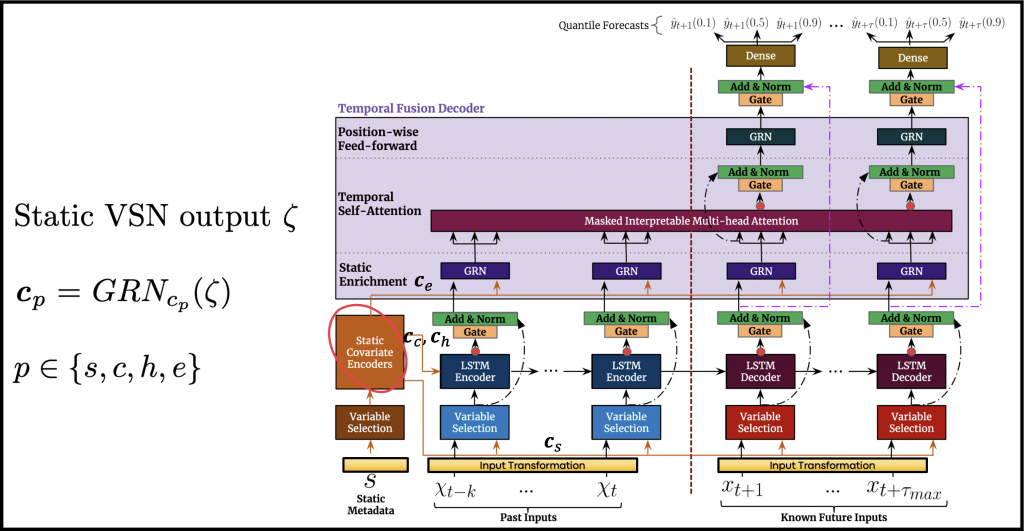
return outputs, sparse_weightsStatic Covariates Encoding
As opposed to other time-series forecasting methods, this model was designed to intrinsically integrate the information coming from the static inputs. The static information is crucially important, but is often discarded by other methods, or used inefficiently.
The integration is achieved using four different GRNs applied to the static VSN’s output. The GRNs generate separate context signals that help to propagate the static information into deeper stages of processing.
- \(\boldsymbol{c_{s}}\) – refers to the context signal fed to the VSN blocks operating on the temporal input channels.
- \(\boldsymbol{c_{c}}\) and \(\boldsymbol{c_{h}}\) – are used as the initial cell state and hidden state of the recurrent layer, which will be described in the next sub-section. As a result, every observation will be processed using different initial cell and hidden states.
- \(\boldsymbol{c_{e}}\) – is the context signal used for the static enrichment phase, applied to the processed sequences at a later stage of processing.
In terms of implementation, all that is required is to initialize these GRNs, which represent the static encoders, as part of the constructor of the complete TFT class:
# =============================
# static covariate encoders
# =============================
static_covariate_encoder = GatedResidualNetwork(input_dim=self.state_size,
                                                hidden_dim=self.state_size,
                                                output_dim=self.state_size,
                                                dropout=self.dropout)
self.static_encoder_selection = copy.deepcopy(static_covariate_encoder)
self.static_encoder_enrichment = copy.deepcopy(static_covariate_encoder)
self.static_encoder_sequential_cell_init = copy.deepcopy(static_covariate_encoder)
self.static_encoder_sequential_state_init = copy.deepcopy(static_covariate_encoder)
Sequence-to-sequence Processing
The goal of the sequence-to-sequence processing phase is to generate features that are dependent on the local context in the temporal data. Such processing utilizies the local connection between steps that are close in time.
The outputs of the VariableSelectionNetworks applied to the temporal input channels, denoted as \(\boldsymbol{\tilde{\xi}}_{t}\), are fed into dedicated LSTM modules:
- The processed historical time-series are fed to the recurrent module denoted as Encoder. As implied earlier, \(\boldsymbol{c_{c}}\) and \(\boldsymbol{c_{h}}\), output by the static covariate encoders, are used to initialize the
cell_stateandhidden_stateof the Encoder. - The
cell_stateandhidden_stateassociated with the last historical time-step are fed into a separate recurrent layer, denoted as Decoder. Its input is composed of the processed future time-series.
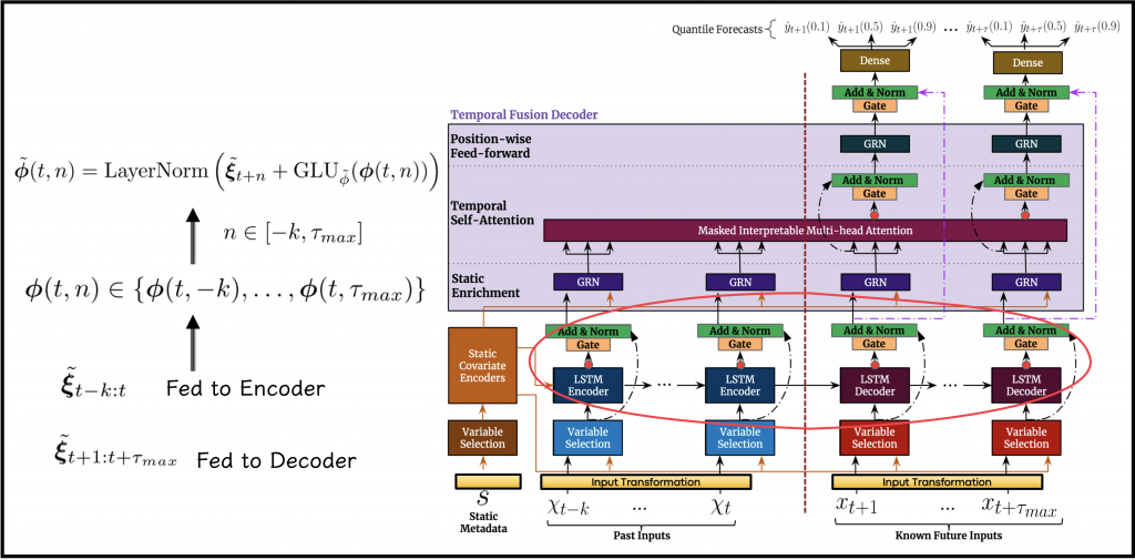
As a result of this processing, the next step will hopefully have access to a uniform set of temporal variables, denoted as \(\boldsymbol{\phi}(t,n)\). A gating operation and a residual by-pass connection are applied to \(\boldsymbol{\phi}(t,n)\), allowing the model to attenuate some of the complexity, resulting in \(\boldsymbol{\tilde{\phi}}(t,n)\)
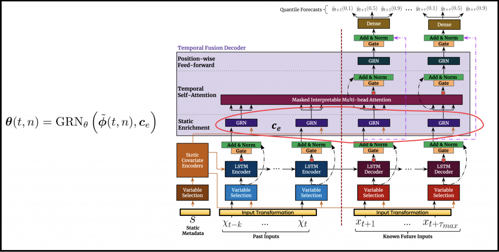
Static Enrichment
An additional phase of non-linear processing is termed StaticEnrichment. In this phase, the static covariates are used to enhance the learned temporal features. This is achieved by feeding the output of the sequence-to-sequence processing stage into an additional GRN. The context input of the additional GRN is the signal \(\boldsymbol{c_{e}}\), which is provided by the static covariate encoders. The resulting temporal sequence is denoted as \(\boldsymbol{\theta}(t,n)\).
Self-Attention
The last interesting part of the model’s architecture is the self-attention mechanism. This mechanism is designed to assist the model in learning long-term relationships between points in time. In addition, a modification made by the authors to the common multi-head attention mechanism enables us to use the scores computed by this mechanism as explanatory outputs, which will be covered below.
In general, attention mechanism receives three tensors as inputs: Queries – denoted as \(\boldsymbol{Q}_{N \times d_{attn}}\), Keys – denoted as \(\boldsymbol{K}_{N \times d_{attn}}\) and Values – denoted as \(\boldsymbol{V}_{N \times d_{v}}\). Its output is the multiplication of the Values tensor by the outcome of a function, \(A\), applied to \(\boldsymbol{Q}\) and \(\boldsymbol{K}\):
\(\mathrm{Attention}(\boldsymbol{Q},\boldsymbol{K},\boldsymbol{V}) = A(\boldsymbol{Q},\boldsymbol{K})\boldsymbol{V}\)
A common choice for the function \(A\) is the scaled dot-product attention, defined as follows:
\(A(\boldsymbol{Q},\boldsymbol{K})=\mathrm{Softmax}(\boldsymbol{Q}\boldsymbol{K}^{T} / \sqrt{d_{attn}})\)
Multi-head self-attention achieves greater learning capacity by maintaining parallel and separate attention mechanisms that yield different representations. To do so, in the case of \(m_H\) heads, for each head \(h\), the model will hold a separate set of learned projection matrices:
\(\boldsymbol{W}^{(h)}_{K} \epsilon \mathbb{R}^{d_{model} \times d_{attn}} , \boldsymbol{W}^{(h)}_{Q} \epsilon \mathbb{R}^{d_{model} \times d_{attn}}, \boldsymbol{W}^{(h)}_{V} \epsilon \mathbb{R}^{d_{model} \times d_{V}}\)
Each head separately applies the associated set of projection weights as follows:
\(\boldsymbol{H}_{h} = \mathrm{Attention}(\boldsymbol{Q}\boldsymbol{W}^{(h)}_{Q},\boldsymbol{K}\boldsymbol{W}^{(h)}_{K},\boldsymbol{V}\boldsymbol{W}^{(h)}_{V})\)
Eventually, the different \(m_H\) heads are concatenated and projected, by multiplying with the learned set of weights \(\boldsymbol{W}_{H} \epsilon \mathbb{R}^{(m_{H} \cdot d_{V}) \times d_{model}}\), as follows:
\(\mathrm{MultiHead}(\boldsymbol{Q},\boldsymbol{K},\boldsymbol{V}) = [\boldsymbol{H}_{1},…,\boldsymbol{H}_{m_{H}}]\boldsymbol{W}_{H}\)
On top of the Multi-Head Self-Attention module, the authors suggest a modification they term InterpretableMultiHead Attention. As opposed to traditional multi-head self-attention, in which the Values are projected differently for each separate head, in the new mechanism, the projected Values are shared across heads. This means that, instead of having a separate \(\boldsymbol{W}^{(h)}_{V}\) for each head, we maintain just a single, shared \(\boldsymbol{W}_{V}\). The different heads simply take care of the interactions between the Queries and the Keys, and the outputs of the heads are aggregated and averaged before multiplying by the projected values:
\(\mathrm{InterpretableMultiHead}(\boldsymbol{Q},\boldsymbol{K},\boldsymbol{V}) = \tilde{\boldsymbol{H}}\boldsymbol{W}_H\)
where \(\tilde{\boldsymbol{H}}\) is defined as follows:
\(\tilde{\boldsymbol{H}} = \tilde{A}(\boldsymbol{Q},\boldsymbol{K})\boldsymbol{V}\boldsymbol{W}_{V}\)
\( = \{ \frac{1}{m_H} \sum_{h=1}^{m_H}A((\boldsymbol{Q}\boldsymbol{W}^{(h)}_{Q},\boldsymbol{K}\boldsymbol{W}^{(h)}_{K})\}\boldsymbol{V}\boldsymbol{W}_{V}\)
\( = \frac{1}{m_H} \sum_{h=1}^{m_H} \mathrm{Attention} ((\boldsymbol{Q}\boldsymbol{W}^{(h)}_{Q},\boldsymbol{K}\boldsymbol{W}^{(h)}_{K}\boldsymbol{V}\boldsymbol{W}_{V})\)
As in plain multi-head self-attention, here too, every head can learn different temporal patterns. However, unlike plain multi-head self-attention, all the heads access a common set of features contained in \(\boldsymbol{V}\boldsymbol{W}_{V}\). In addition, \(\tilde{A}(\boldsymbol{Q},\boldsymbol{K})\) is considered as an ensemble of attention scores or weights.
In practice, in the context of TFT, the InterpretableMultiHead Attention module is fed with the static enrichment stage’s output, \(\boldsymbol{\Theta}(t) \epsilon \mathbb{R}^{N \times total\_steps \times state\_size}\), where \(N\) indicates the number of samples (possibly the size of the batch), \(total\_steps\) is the number of time-steps to consider, including the historical time-window and the set of future horizons, and \(state\_size\) is the hyperparameter controlling the architecture.
\(\boldsymbol{\Theta}(t)\) is treated by the InterpretableMultiHead Attention module as the Queries, the Keys, and the Values (as implied by the diagram in Figure 8). In practice, only the Queries that correspond to the future time-steps are the ones that matter. Similarly, we only regard the time-steps which come later than \(t\), when we continue to process the output of the module, denoted as \(\boldsymbol{B}(t)\).
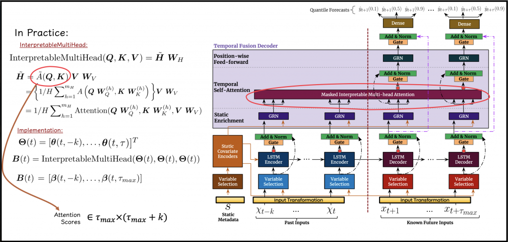
Moreover, in the same attention mechanism, we perform decoder masking. The masking is used to ensure that every future time-step is only exposed to information that was observed before the current step, hence, ensuring that the streaming of information towards the prediction is causal.
In terms of explanatory outputs, \(\tilde{A}(\boldsymbol{Q},\boldsymbol{K})\) is used as a scoring function between a future-horizon (a time-step into the future), and another time-step. The provided score is supposed to quantify the influence of one time-step for the prediction of a future time-step in question. Hence, these scores allow us to gain insights regarding the time-steps that most significantly affected the model’s outputs. As opposed to more traditional models for time-series analysis, which require ad-hoc specification in advance of concepts such as seasonality, trend, and so on, the TFT model can learn these patterns on its own.
The following is a possible implementation of the InterpretableMultiHead Attention module :
class InterpretableMultiHeadAttention(nn.Module):
    """
    The mechanism implemented in this module is used to learn long-term relationships across different time-steps.
    It is a modified version of multi-head attention, for enhancing explainability. On this modification,
    as opposed to traditional versions of multi-head attention, the "values" signal is shared for all the heads -
    and additive aggregation is employed across all the heads.
    According to the paper, each head can learn different temporal patterns, while attending to a common set of
    input features which can be interpreted as  a simple ensemble over attention weights into a combined matrix, which,
    compared to the original multi-head attention matrix, yields an increased representation capacity in an efficient
    way.

    Parameters
    ----------
    embed_dim: int
        The dimensions associated with the ``state_size`` of th model, corresponding to the input as well as the output.
    num_heads: int
        The number of attention heads composing the Multi-head attention component.
    """

    def __init__(self, embed_dim: int, num_heads: int):
        super(InterpretableMultiHeadAttention, self).__init__()

        self.d_model = embed_dim  # the state_size (model_size) corresponding to the input and output dimension
        self.num_heads = num_heads  # the number of attention heads
        self.all_heads_dim = embed_dim * num_heads  # the width of the projection for the keys and queries

        self.w_q = nn.Linear(embed_dim, self.all_heads_dim)  # multi-head projection for the queries
        self.w_k = nn.Linear(embed_dim, self.all_heads_dim)  # multi-head projection for the keys
        self.w_v = nn.Linear(embed_dim, embed_dim)  # a single, shared, projection for the values

        # the last layer is used for final linear mapping (corresponds to W_H in the paper)
        self.out = nn.Linear(self.d_model, self.d_model)

    def forward(self, q, k, v, mask=None):
        num_samples = q.size(0)

        # Dimensions:
        # queries tensor - q: [num_samples x num_future_steps x state_size]
        # keys tensor - k: [num_samples x (num_total_steps) x state_size]
        # values tensor - v: [num_samples x (num_total_steps) x state_size]

        # perform linear operation and split into h heads
        q_proj = self.w_q(q).view(num_samples, -1, self.num_heads, self.d_model)
        k_proj = self.w_k(k).view(num_samples, -1, self.num_heads, self.d_model)
        v_proj = self.w_v(v).repeat(1, 1, self.num_heads).view(num_samples, -1, self.num_heads, self.d_model)

        # transpose to get the following shapes
        q_proj = q_proj.transpose(1, 2)  # (num_samples x num_future_steps x num_heads x state_size)
        k_proj = k_proj.transpose(1, 2)  # (num_samples x num_total_steps x num_heads x state_size)
        v_proj = v_proj.transpose(1, 2)  # (num_samples x num_total_steps x num_heads x state_size)

        # calculate attention using function we will define next
        attn_outputs_all_heads, attn_scores_all_heads = self.attention(q_proj, k_proj, v_proj, mask)
        # Dimensions:
        # attn_scores_all_heads: [num_samples x num_heads x num_future_steps x num_total_steps]
        # attn_outputs_all_heads: [num_samples x num_heads x num_future_steps x state_size]

        # take average along heads
        attention_scores = attn_scores_all_heads.mean(dim=1)
        attention_outputs = attn_outputs_all_heads.mean(dim=1)
        # Dimensions:
        # attention_scores: [num_samples x num_future_steps x num_total_steps]
        # attention_outputs: [num_samples x num_future_steps x state_size]

        # weigh attention outputs
        output = self.out(attention_outputs)
        # output: [num_samples x num_future_steps x state_size]

        return output, attention_outputs, attention_scores

    def attention(self, q, k, v, mask=None):
        # Applying the scaled dot product
        attention_scores = torch.matmul(q, k.transpose(-2, -1)) / math.sqrt(self.d_model)
        # Dimensions:
        # attention_scores: [num_samples x num_heads x num_future_steps x num_total_steps]

        # Decoder masking is applied to the multi-head attention layer to ensure that each temporal dimension can only
        # attend to features preceding it
        if mask is not None:
            # the mask is broadcast along the batch(dim=0) and heads(dim=1) dimensions,
            # where the mask==True, the scores are "cancelled" by setting a very small value
            attention_scores = attention_scores.masked_fill(mask, -1e9)

        # still part of the scaled dot-product attention (dimensions are kept)
        attention_scores = F.softmax(attention_scores, dim=-1)
        # matrix multiplication is performed on the last two-dimensions to retrieve attention outputs
        attention_outputs = torch.matmul(attention_scores, v)
        # Dimensions:
        # attention_outputs: [num_samples x num_heads x num_future_steps x state_size]

        return attention_outputs, attention_scores
We initialize this module upon the construction of the TFT object:
self.multihead_attn = InterpretableMultiHeadAttention(embed_dim=self.state_size, num_heads=self.attention_heads)then apply it to the static enrichment phase’s output, while specifying the masking tensor:
# create a mask - so that future steps will be exposed (able to attend) only to preceding steps
output_sequence_length = num_future_steps - self.target_window_start_idx
mask = torch.cat([torch.zeros(output_sequence_length,
                              num_historical_steps + self.target_window_start_idx,
                              device=enriched_sequence.device),
                  torch.triu(torch.ones(output_sequence_length, output_sequence_length,
                                        device=enriched_sequence.device),
                             diagonal=1)], dim=1)
# Dimensions:
# mask: [output_sequence_length x (num_historical_steps + num_future_steps)]

# apply the InterpretableMultiHeadAttention mechanism
post_attention, attention_outputs, attention_scores = self.multihead_attn(
    q=enriched_sequence[:, (num_historical_steps + self.target_window_start_idx):, :],  # query
    k=enriched_sequence,  # keys
    v=enriched_sequence,  # values
    mask=mask.bool())
# Dimensions:
# post_attention: [num_samples x num_future_steps x state_size]
# attention_outputs: [num_samples x num_future_steps x state_size]
# attention_scores: [num_samples x num_future_steps x num_total_steps]
Wrapping Up
After applying the attention mechanism, the remaining steps are quite straight-forward (see Figure 8):
- Gating and residual connections to the static enrichment outputs.
- An additional GRN is distributed across the temporal sequence.
- Gating and residual connection to the outputs of the sequence-to-sequence processing layer.
- Finally, the estimated quantiles for each horizon are acquired through the application of linear layers. The output dimension of the linear layers is configured according to the number of desired quantiles.
The complete implementation of the TemporalFusionTransformer class is available in the tft_torch repository / package. This class represents the complete model and defines the information flow between the blocks that were explained in this post.
According to the paper’s reported results, TFT outperforms all the other state-of-the-art benchmarks, on a wide variety of tasks and datasets. In predicting the median, for example, the TFT gets losses lower by 7% from the next best model. In the authors’ perspective, this emphasizes the benefits of adapting the architecture to the generic formulation of a prediction problem of this kind.
As demonstrated in the usage tutorials, for building the model only the following parameters require configuration:
- The set of quantiles to be estimated.
- \(d_{model}\) – the embedding width, which dominates most of the architecture’s properties.
- \(m_{H}\) – the number of attention heads.
- The number of levels in the stack of recurrent layers (on the sequence-to-sequence processing phase).
- The dropout rate.
Such a small set of hyperparameters, which determines the entire structure of the model, renders the usage of this model even more appealing.
Interpretable Outputs
As elaborated in this post, the TFT model generates tensors that can be used to better understand model performance and explain its estimations. Hence, the most useful outputs of the model, except for the predicted quantiles, of course, are the selection weights, denoted as \(\nu_{\chi_{t}}\), and the attention scores, denoted as \(\tilde{A}(\boldsymbol{Q},\boldsymbol{K})\).
The specific illustrations provided in this section refer to the Corporación Favorita Grocery Sales dataset. A guide for pre-processing this dataset into a suitable structure is provided in the tutorials[BROKEN_LINK] section of tft-torch.
Let us assume a use-case in which the evaluated model, was trained to estimate a set of \(d_q\) quantiles, using a subset including \(N\) observations. Each observation consists of:
- a historical time-series that includes \(m_x\) temporal variables, spanning \(k\) past time-steps.
- a futuristic time-series including \(m_{χ}\) temporal variables, spanning \(\tau_{max}\) time steps.
- a set of \(m_s\) static variables.
The output of the model implemented in tft-torch, includes the following tensors, which can be aggregated batch-by-batch to form arrays to represent the evaluation of an entire subset:
predicted_quantiles– the model quantile estimates for each temporal future step, shaped as \([N \times \tau_{max} \times d_q]\).static_weights– the selection weights associated with the static variables for each observation, shaped as \([N \times m_s]\).historical_selection_weights– the selection weights associated with the historical temporal variables, for each observation, and past time-step, shaped as \([N \times k \times m_x]\).future_selection_weights– the selection weights associated with the future temporal variables, for each observation, and future time-step, shaped as \([N \times \tau_{max} \times m_χ]\).attention_scores– the attention score each future time-step associates with each other time-step, for each observation, shaped as \([N \times \tau_{max} \times (k + \tau_{max})]\).
These outputs can be used for interpretation purposes on a single sample-level (examining the outputs of a single observation), or on a subset-level, where we aggregate the outputs of the entire subset.
Selection Weights
Recall that the TFT model has a separate internal mechanism of variable selection (VSN) for each information channel.
Note that both the categorical and the numerical variables of the channel are concatenated together after the input transformation phase. Thus, VSN acts on them in the same manner.
For subset level description, we are required to perform some kind of reduction/aggregation of the weights computed for the entire subset. For that matter, as suggested by the paper, we use a set of percentiles (which are not related whatsoever to the estimated quantiles of the target variable), for describing the distribution of selection weights for each variable on each input channel.
Using tft_torch.visualize [BROKEN_LINK] on a validation set from the Corporación Favorita Grocery Sales dataset, we can generate the following description:
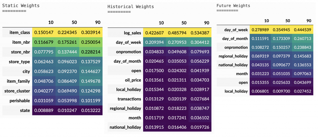
The tables in Figure 9 display the specified percentiles (in this case: 10,50 and 90) of each feature’s weight distribution, on each input channel. The color of each cell is highlighted according to the corresponding value, where brighter color implies a higher value. Note that for the temporal inputs (historical/futuristic time-series), the sequence of weights corresponding to each time-step is “flattened“, so that the aggregation is performed along time-steps and samples likewise.
These illustrations are, of course, specific to the mentioned Favorita dataset, but can also shed light on the potential usage of such outputs. Some interesting findings from the tables point to the fact that:
- The attributes that seem to have the highest weights (among the static inputs channel) and are, therefore, considered more important, are those that are associated with the identity of the instance –
store_nbr,item_nbranditem_class. - The most important variable among the historical features – in terms of selection weight – is the target variable the model was trained to predict into the future,
log_sales, which makes perfect sense. This finding can serve as a sanity check. - Among the known (futuristic) inputs, we see that prior knowledge about the next weekdays and the upcoming promotions is of high importance to the model.
As noted earlier, we can examine the selection weights from an individual sample perspective (as demonstrated in the tutorial). Doing so enables us to investigate specific samples, for which the model either performed extremely well or failed miserably, and understand which variables of the specific sample more significantly affected the model and led to the un/successful prediction.
Attention Scores
The TFT model also has an internal mechanism for weighting the information coming from the sequential data, whether it is the historical or the future sequence. The output attention_scores , provided by the model, can be used to infer which preceding time-steps affected the model’s output the most. Recall that due to masking, each future horizon can only “assign” attention to preceding steps.
The attention scores are horizon-specific, i.e. every future horizon maintains a different set of scores for the corresponding observed time-steps. As suggested in the paper, and using the visualization utilities provided as part of tft-torch, we can examine the attention score for a one-step horizon, \((t+1)\), into the future:
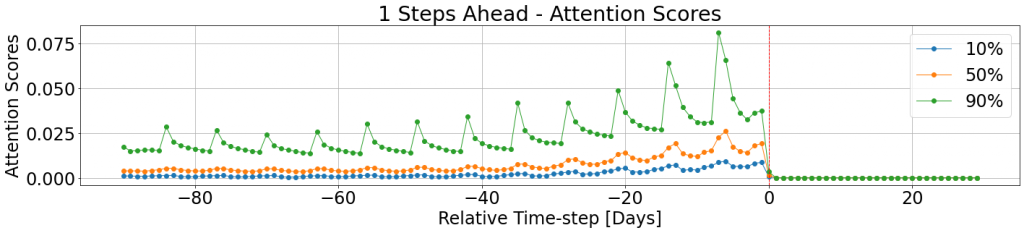
The dashed line indicates the separation between the historical and the futuristic time-steps. To describe the attention patterns across the entire subset in hand, we compute percentiles of the attention scores associated with the selected horizon. The attention scores for the further time-steps are zeroed out by design, using the internal decoder masking applied as part of the model. The Corporación Favorita Grocery Sales dataset contains retail data, which goes hand-in-hand with the 7-days cycle we see in the attention scores. Moreover, one can notice the general trend, according to which the most recent cycles (the ones that are closer to the separation line), are more dominant than previous, gradually forgotten, cycles.
Such an illustration can also be used to visualize the attention scores patterns for multiple horizons at once:
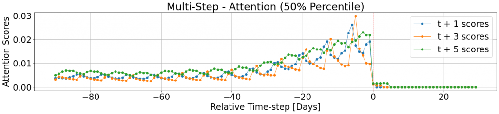
For example, in Figure 11, one can see that the attention scores for the historical time-steps share characteristics across the different horizons. They are all decaying towards the past and have weekly cycles, but, these weekly cycles are offset, due to the difference in weekdays. Moreover, we see that in this case future steps preceding the selected horizon are not assigned high attention scores, even when unmasked.
As for the selection weights, attention scores can also be evaluated on a single-sample level (also demonstrated in the tutorial). Doing so enables the investigation of specific samples, for which the model performed extremely well / failed miserably, and understanding which time-steps strengthened/fooled the model.
Quick Summary
These two posts cover the work presented in the paper “Temporal Fusion Transformers for Interpretable Multi-horizon Time Series Forecasting”1, by Bryan Lim, Sercan O. Arik, Nicolas Loeff, and Tomas Pfister. They provide a general description of the problems for which multi-horizon forecasting can be beneficial, and a formulation of the optimization task, according to which the TemporalFusionTransformer model is trained.
In addition, these posts elaborate on the model’s structure and architecture and provide a possible implementation for said model (available as part of tft-torch). Finally, possible model outputs uses were demonstrated.
In our experience, the virtues of the TemporalFusionTransformer model, besides state-of-the-art predictive performance, are tremendous, :
- Allows for the “packing” of estimates for multiple horizons, using a single model.
- Opens the door to out-of-the-box uncertainty bounds, embodied by the multiple quantile estimates.
- Empowers easily-retrieved explanatory outputs; the selection weights and attention scores.