Multi-horizon Forecasting using Temporal Fusion Transformers – A Comprehensive Overview – Part 1
By Dvir Ben Or and Michael Kolomenkin
Time-series forecasting is a problem of major interest in many business domains, such as finance, weather, and others. This problem is challenging for several reasons. First, forecasting often requires the consideration of a wide set of diverse variables of different nature. Combining all these variables, which can span multiple input sources, is a complex task. Second, it is often desired to predict the target signal for several future points in time. For instance, in weather forecasting, it is preferable that the weather be estimated for several days ahead, each and every day. Third, the predictive outcome of the forecasting model needs to be interpretable by a human. Interpretability is critical for decision-making.
A paper by Bryan Lim, Sercan O. Arik, Nicolas Loeff, and Tomas Pfister (from Oxford University and Google Cloud), named “Temporal Fusion Transformers for Interpretable Multi-horizon Time Series Forecasting”1, suggests a detailed solution for such problems. We re-implemented the original TensorFlow implementation in PyTorch and added examples.
In the next two blogposts we will provide a step-by-step overview of the solution suggested in the said paper, as well as the new approach they present, accompanied by code demonstrations. We hope these will help clarify the core ideas presented by the authors.
The first post describes the Multi-Horizon Forecasting (MHF) problem and the scenarios in which MHF is beneficial in detail, outlines the advantages of the Temporal Fusion Transformer (TFT) for MHF, and formally defines the optimization task used for training the TFT. The second post details the model’s structure and implementation and demonstrates how its outputs can be used for further analysis.
Multi-Horizon Forecasting
Multi Horizon Forecasting provides information on the target variable at multiple future points in time. Providing access to estimates of the target variable along a future trajectory can provide users with great value, allowing them to optimize their actions at multiple steps. For example, retailers can use estimates of future sales to optimize their supply chain and promotions, investment managers can leverage the forecasting of the future financial asset prices to maximize their portfolio’s performance, and healthcare institutions can use the predicted number of future patient admissions to ensure they have sufficient personal and equipment at the ready.
Practical MHF use-cases involve a variety of data sources, including:
- Static metadata – All the non-temporal information associated with the observation, such as the user’s gender, the store’s location, or the product category, depending on the dataset properties.
- Historical exogenous time-series – Past values of multiple temporal variables, Usually including the target variable as well.
- Future time-series – Known information about the future. These are temporal inputs that can be specified in advance, such as a planned promotion for a specific day, upcoming holiday, or relevant weekday, for each future time step.
In addition, some of the temporal features and the static attributes involved can be numerical, while others can be categorical. However, usually there is no prior knowledge of how these sources interact or how they might affect the target variable.
As such, the author’s goal for this study, beyond accurate predictions (which is stating the obvious), is:
- To suggest a tool or model that would allow the processing of the heterogeneous data channels that are usually available in MHF use cases.
- To provide methods for interpreting and explaining the outputs of such a model.
TFT Advantages
Before diving into the details of model composition and its objective function, let us go over the advantages of the TFT model over earlier methods.
- The inductive bias of the architecture – Most of the existing solutions for MHF, employ assumptions that are either violated in actual multi-step time-series forecasting scenarios or do not utilize effectively the available information.
For example, autoregressive models commonly assume that the non-target temporal variables, also termed as exogenous inputs, are all known, going into the future. However, this is rarely the case in practice. In most real-life scenarios, temporal variables are not all known in advance.
Other methods neglect the static attribute inputs, or their essence, by simply concatenating them with the temporal inputs. Thus, the static information is not utilized effectively.
According to Wikipedia, an inductive bias of a learning algorithm refers to the assumptions that the learner uses to predict outputs of inputs that have not been encountered. Injection of inductive bias into the phase of model architecture design, so that the process considers the characteristics and structure of the relevant data, is what yielded substantial progress both in time-series modeling and in the general deep learning domain in general.
Correspondingly, the TFT has an integral ability to process the different channels of information that are commonly available in typical MHF use cases. - Out-of-the-box explainability – Existing methods in this domain are often treated as ‘black-boxes’. They contain complex connections and interactions between a great number of parameters, in a way that makes it difficult to explain the model’s outputs. An inability to interpret the outputs makes it difficult to gain the end-user’s trust, with respect to these outputs.
Commonly used explainability methods (such as LIME or SHAP), in their general, more-known form, are not suited to time-series modeling, as they do not take into account the temporal characteristics of the data.
Rather, attention-based methods (such as transformers) enable to place emphasis and quantify the importance of specific time-steps for the modeling task, but cannot be used for quantifying the importance of individual input features.
The authors of the paper bridge this explainability gap, by designing a single model that simultaneously enables:
– The identification of variables that are significant globally, i.e. across the entire dataset.
– The identification of temporal patterns that characterize the dataset.
– Instance-wise interpretability, both in terms of variables importance and in terms of emphasizing significant points in time.
Later in the post, we show how such explainability is achieved, using some examples.
Notations & Formulation
Previously, we presented the MHF task and explained the advantages of the TFT approach. Now, let us define the problem formally. For clarity purposes, some of the notations are a bit different from those presented in the paper.
Let us assume a dataset, in which each entity, or observation, indexed by \(i\), is associated with a corresponding sequence of target values, \(y_{i,t} \epsilon \mathbb{R}\), where \(t \epsilon [0, T_{i}]\) are future time-steps, and \(T_{i}\) indicates the maximal horizon (in time-steps) for the \(i\)-th observation.
In terms of inputs, the \(i\)-th observation is associated with:
- \(\mathbf{s}_{i} \epsilon \mathbb{R}^{m_{s}}\) – denoting the set of \(m_{s}\) static attributes.
- \(\mathbf{χ}_{i,t} \epsilon \mathbb{R}^{m_{χ}}\) – denoting the historical time-series, including the observed temporal attributes. Each of the \(m_{χ}\) attributes composing this input channel are included for each of the historical time-steps. Let us use \(k\) to denote the historical time-window length, in time-steps.
- \(\mathbf{x}_{i,t} \epsilon \mathbb{R}^{m_{x}}\) – denoting the future time-series, including the known temporal attributes to which we have access for each future point in time, e.g. the day of the week. Each of the \(m_{x}\) attributes composing this input channel are included for each of the future time-steps.
Remember that in practice, each of these input information channels can include both numeric attributes and categorical attributes. Hence, each training batch is composed as follows:
In [1]: list(batch.keys())
Out [1]: ['target',
 'static_feats_numeric',
 'static_feats_categorical',
 'historical_ts_numeric',
 'historical_ts_categorical',
 'future_ts_numeric',
 'future_ts_categorical']
Optimization
In this section, we describe the function that the TFT is trained to optimize.
In most of the cases in which MHF is required, access to prediction intervals can be useful for decision optimization and risk management. For example, in weather forecasting, instead of predicting that “temperature will be 20 degrees Celcius”, the model will predict that “temperature will be in the range between 17 and 23 degrees Celcius, with a probability of 90%”. Prediction intervals can, therefore, be used to estimate the best and worst-case scenarios.
Formally, prediction intervals are achieved via quantile regression. The model can be configured to simultaneously predict some percentiles (e.g. the 10th, 50th, and the 90th) of the target variable.
The output of the model is a function of the desired quantile and the future horizon time-step, which takes as input the information channels specified above:
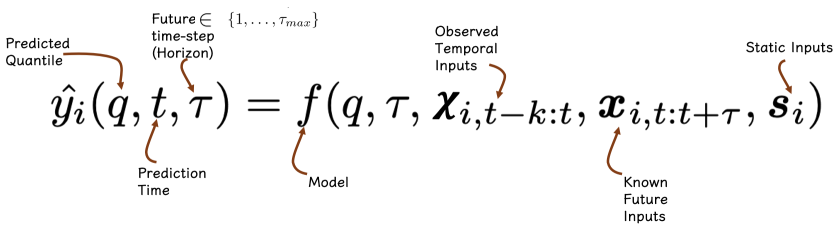
Practically, the model simultaneously outputs its predictions for all the desired quantiles and horizons.
The model is trained to optimize the following objective function:
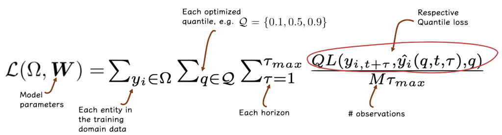
where \(\Omega\) refers to the subset, containing \(M\) observations, according to which the loss is computed, \(\tau_{max}\) is the maximal (furthest) horizon considered, \(W\) is the set of model parameters, and \(\mathcal{Q}\) is the set of quantiles to be estimated.
Each combination of observation, future horizon, and quantile requires the computation of the quantile loss function, denoted by \(QL\) (to be described shortly). As implied by the equation, these computations are then averaged across observations and horizons.
Quantile Loss Function
The quantile loss function is defined as:
\( QL(y,\hat{y},q) = q(y-\hat{y})_{+} + (1-q)(\hat{y}-y)_{+} \)
where \((\cdot)_+ = \mathrm{max}(0,\cdot)\) is a rectifying function that caps any negative value with zero, and \(q \epsilon [0,1]\).
A bit of intuition:
- If the estimate, \(\hat{y}\), is lower than the target value, \(y\), we are left only with the left part of the expression, as the right part gets zeroed out. If the configured quantile is low (small value of \(q\)), the contribution to the loss is small, due to the multiplication by \(q\)), which is small. On the other hand, if the configured quantile, \(q\)), is high, the multiplication by q yields a higher contribution to the loss.
- In contrast, if the estimate, \(\hat{y}\), is higher than the target value, then only the right part of the expression is relevant. In this case, if the configured quantile is low (small value of \(q\)) then the multiplication by \((1-q)\) would increase the contribution to the loss. Similarly, if the quantile \(q\) is set to a higher value, the contribution to the loss decreases.
Refer to this page for a deeper understanding of why such a loss function converges into the optimization of an estimator for a specific quantile \(q\).
Note that quantile optimization is not exclusive to the Temporal Fusion Transformer model; it can be applied anywhere. In practice, it can be computed in another form, because the two parts of the expression in the loss function cannot both be non-zero at once. Hence, \( QL\) can be also be formulated as follows:
\( QL(y,\hat{y},q) = \mathrm{max}((q-1) \cdot errors , q \cdot errors )\)
where \( errors = y – \hat{y} \).
A possible implementation, also available as part of tft-torch, is as follows:
import torch


def compute_quantile_loss_instance_wise(outputs: torch.Tensor,
                                        targets: torch.Tensor,
                                        desired_quantiles: torch.Tensor) -> torch.Tensor:
    """
    This function compute the quantile loss separately for each sample,time-step,quantile.

    Parameters
    ----------
    outputs: torch.Tensor
        The outputs of the model [num_samples x num_horizons x num_quantiles].
    targets: torch.Tensor
        The observed target for each horizon [num_samples x num_horizons].
    desired_quantiles: torch.Tensor
        A tensor representing the desired quantiles, of shape (num_quantiles,)

    Returns
    -------
    losses_array: torch.Tensor
        a tensor [num_samples x num_horizons x num_quantiles] containing the quantile loss for each sample,time-step and
        quantile.
    """

    # compute the actual error between the observed target and each predicted quantile
    errors = targets.unsqueeze(-1) - outputs
    # Dimensions:
    # errors: [num_samples x num_horizons x num_quantiles]

    # compute the loss separately for each sample,time-step,quantile
    losses_array = torch.max((desired_quantiles - 1) * errors, desired_quantiles * errors)
    # Dimensions:
    # losses_array: [num_samples x num_horizons x num_quantiles]

    return losses_array
This function will compute the quantile loss associated with each observation, quantile, and horizon, respectively. For aggregating all the contributions to the loss on a dataset level, we can use the following:
losses_array = compute_quantile_loss_instance_wise(outputs=outputs,
                                                   targets=targets,
                                                   desired_quantiles=desired_quantiles)

# sum losses over quantiles and average across time and observations
q_loss = (losses_array.sum(dim=-1)).mean(dim=-1).mean()  # a scalar (shapeless tensor)
Conclusion
This post overviewed the domain of problems that the Temporal Fusion Transformer aims to tackle, as well as the formulation of such problems, the characteristic inputs that are commonly available, and the optimization task performed by the model.
The next post will provide a detailed description of the model itself, accompanied by code.