By Ofer Shapira and Dan Halbersberg

Digital advertising plays a significant role in generating income for many online companies. According to Statista, global digital advertising spending will exceed 600$ billion by 2023. To maximize their revenue, many companies aim to automate their investments in digital media buying.

In this blog post, we present a budget allocation method that leans on a small set of prior assumptions, making it robust in face of the wide diversity of advertisement methods. Namely, this blog presents a two-step budget allocation method: Model the fundamental investment-return relation, then optimally allocate the budget.

Reading this technical blog post, will teach you about the problem and challenges, and will offer you a step-by-step understanding of our solution and assumptions.

Background

The concept of “spending money to make money” governs various aspects of our lives. Whether it’s a student investing in tuition fees for education and subsequent job prospects, or a company allocating resources for research and development to generate revenue, the process involves multiple steps. Our objective is to develop an algorithm that focuses on the ultimate events of spending and earning money, abstracting away the specific details that govern this transformation. This approach allows our algorithm to be applicable to a diverse range of processes, capturing the conversion of costs into returns across various contexts.

We focus our attention on the task of budget allocation, specifically in the realm of online advertising for mobile users. This platform presents a twofold challenge. On one hand, it limits advertiser control as ads may traverse a complex network of external vendors managing communication between the advertiser and the publisher, offering various presentation options for products. On the other hand, it provides an opportunity for tracking the performance of actions. This includes valuable insights on metrics such as the number of installs, revenue generated, and user retention, all while considering the associated costs.

Problem Formulation

We treat budget allocation as a constrained optimization problem. This requires us to define the following essential elements:

1. Decision variables
2. The objective
3. Constraints

We consider the costs as our decision variables. Each cost investment (“money-out”) leads to a return, typically in the form of revenue (“money-in”) or other measures of engagement with our product. For instance, in the case of a mobile app, we may measure user activity such as the number of days logged in or specific actions taken within the app. We use the term “key performance indicator” (KPI) as a general standard to represent the measurement used to quantify our returns. Our objective is to maximize the overall return from our investment. We also have a global constraint that ensures the total sum of costs remains within the available budget. Local constraints may further restrict the cost range for each decision variable.

We mentioned that the decision variables represent investment costs, but who owns these costs? It is tempting to assign them to individual “users,” as they are the smallest units we pay for and expect returns from. However, this is rarely the case, for several reasons.

First, the ad network typically limits the advertiser’s targeting capability to a small set of properties. For example, marketing campaign may target all Android-US residing in the US, meaning that the investment is essentially made in (Android, US), resulting in the acquisition of a random population of users.

Second, the hierarchical nature of media buying, involving multiple media sources and multiple campaigns per source, introduces interesting questions about optimal budget allocation at different tiers. For example, a marketing lead may be responsible for determining the budget allocated to a group of campaign managers, with each manager overseeing campaigns for a specific media source. Each campaign manager may then seek recommendations on how to distribute the allocated budget among their campaigns.

Third, by considering a population of users at a given time, we can leverage statistical or machine learning tools to enhance the reliability of predictions.

The last paragraph delves into the identification of user groups, potentially with a hierarchical structure. This leads us to the concept of a property sequence, where a property represents a recorded attribute of a user, such as the operating system (OS), country of origin, or the media source that displayed our ad to the user. By combining these properties, we can define specific user populations. Additionally, we assume a property order that allows us to further split populations into sub-populations. For example, we can consider the group of all (Android, US) users and then refine our observations by separating users acquired on Sundays from those acquired on Mondays within a given week. We label these sub-populations as (Android, US, Sunday) and (Android, US, Monday) respectively.

Regardless of the specific sequence of properties we consider, it is beneficial to specify a sequence with two successive refinements. This approach enables us to partition a user population into sub-populations and then further refine each sub-population.

Let’s define those user-tiers, top-to-bottom, and explain their role in our algorithm:

1. Portfolio: The portfolio represents our top-level group of users and reflects our business goals. To stay within the given budget, we must ensure that the acquisition costs for this user group do not exceed the allocated amount. Our objective is to maximize the collective KPI for this portfolio. This optimization program effectively captures these goals through the global constraint and objective.
2. Business Unit (BU): Our control over maximizing the portfolio’s KPI within its total budget lies in the allocation of this budget among independent business units (BUs). Hence, our decision variables indicate the cost assigned to each considered BU. This refinement of the portfolio is essential due to our underlying assumption that the total budget significantly exceeds the supply available from any single BU. Consequently, we must engage with multiple BUs to fulfill our demand. Not only can the available supply vary across BUs, but also the quality of that supply. For example, certain publishers are mobile apps, facilitating ad presentations to their users as an additional revenue stream. Media sources establish partnerships with specific publishers and facilitate connections between advertisers and those publishers. Some media sources may have closer ties to publishers that align more closely with our goals, resulting in users from these publishers being more engaged with our app compared to others.
3. Cohort: Our BU is the sum of its cohorts, which represent sub-groups of users. We record the cost and KPIs of interest for each cohort. This additional refinement allows us to create a dataset for the BU, where each row corresponds to a single cohort, and the features include the cost and the recorded KPIs. Finally, we fit our BU model to this dataset. While we avoid making assumptions about the selected properties, it is desirable to associate each cohort with a time indicator, such as the install date. This enables our model to describe the cumulative effect of cohort acquisition over time.

The Optimization Program

The following is the precise mathematical formulation of our optimization program. Let \(c_i\) represent the cost of the \(i^{th}\) BU, with \(N\) BUs in total. Let \(B\) represent the total budget.

Assume local cost constraints given by \(B_i^L,B_i^H\), such that \(B_i^L \le c_i \le B_i^H\). Obviously, for all \(i\), we must have \(B_i^L \geq 0\) and \(B_i^H \le B\). Note that choosing \(B_i^L = 0\) and \(B_i^H = B\) deactivates the constraint for source \(i\), hence the specification of the local constraints for all \(i\) is possible without loss of generality. Note also, that we must assume that \(\sum B_i^L \le B\). Otherwise, we would not meet the global constraint. Additionally, \(\sum B_i^H > B\) otherwise, no optimization would be required.

Let \(r_i^k(c_i)\) be the return measured by the KPI \(k\) of BU \(i\) after spending \(c_i\). Assume that \(k\) is linear, in the sense that \(\sum r_i^k(c_i)\) is the returned KPI of our portfolio (this linearity property is also handy at the cohort level, allowing us to easily compute the KPI of a cohort as the sum of its users’ KPI). Let \(K\) denote a set of KPI of interests.

Our goal is to maximize the portfolio’s return averaged over all KPIs. To do so, let \(w_k\) serve as the respective weights, for all \(k \in K\). The role of the weights is first, a scaling factor, to allow a combined multi-KPI objective and second, to set the relative importance of each KPI.

Thus, our optimization program becomes:

\(\max\limits_{c_1,…,c_N} \sum_{k \in K} w_k \cdot \sum_{i=1}^{N} r_i^k(c_i)\)

s.t.

\(\sum_{i=1}^{N}c_i  \le B\)

\(B_i^L \le c_i \le B_i^H \qquad \forall i =1,…,N\)

The only unknown components of this program are the KPI models, \(r_i^k(\cdot)\). If these models were non-linear, then generally speaking, we would not have a closed-form solution for the above program.

Therefore, our modeling of \(r_i\) should:

1. Be a good fit to the BU’s cohorts dataset.
2. Reflect future acquisitions’ dynamics; not necessarily those belonging to past ones.
3. Allow us to efficiently solve the optimization program.

The KPI model

When considering the existence of a dataset and the need to fit a model to it, we typically associate it with some form of deep networks. However, upon closer examination of the objective, our models \(r_i^k\) simply consist of collections of 1-D real functions. They map the cost to the expected KPI, which is not the typical situation in machine learning where numerous input features are assumed. While we could potentially increase the input dimension by considering a common model for all the business units (BUs), this would require the introduction of context variables that identify the source. Consequently, finding a common set of variables to describe all the BUs would be necessary. To ensure the robustness of our algorithm and modeling, it is crucial to avoid this requirement.

Not only is the dimension of our dataset’s features small, but the number of samples is also expected to be limited. For example, if we aim to plan our portfolio spending for the upcoming month and consider daily acquisitions of users for each BU as cohorts, each month would typically contain only about 30 data points. We want to avoid data sparsity by ensuring the cohorts are not too small (as many users may choose not to pay). Typically, we wouldn’t rely on too many past months, perhaps no more than the previous year, due to the highly dynamic and non-stationary nature of the BU’s behavior, influenced by various confounding factors. As a result, our dataset would contain a few hundred rows at most, which limits our ability to utilize models with numerous parameters.

Based on the above considerations, it is advisable to select a well-defined, parameterized family of functions. However, choosing the best-fitting model becomes challenging since the dataset is small and many choices could potentially overfit the data. Decreasing the number of parameters can help mitigate overfitting, but due to the scarcity of data and challenges in assessing world stationarity, evaluating and selecting the optimal model becomes difficult. Instead, drawing inspiration from physics, we introduce physical laws that our model must adhere to, enhancing our immunity to overfitting.

Physical Laws

2. Causality – According to our first law, the acquisition process only starts once we start our spending. Therefore, a cost of zero $ must map to a zero KPI. Mathematically, this means our curve must go through the origin, \(<0,0>\)
3. Time Invariance – Our second law asserts that if we repeat and invest the same cost over a given time period, e.g., a month, then our monthly return will be the same as well. Let’s delve into the rationale behind introducing this rule and its philosophical implications. On one hand, we acknowledged earlier that reality is highly dynamic and may cause our collected data to exhibit non-stationary behavior from one month to another. However, we lack insight into the underlying mechanisms driving this transition. Therefore, our best assumption is to believe that given the same cost stimuli, the response of the BU would repeat itself. Adopting this approach ensures that our model does not predict a better or worse outcome for the next acquisition without any additional information beyond the previous acquisition. Nevertheless, if we do possess additional information, we can incorporate it accordingly. For instance, if seasonal effects suggest that users in the upcoming month are expected to return 10% more than the average user in the current month, we can adjust the KPI column in our dataset accordingly. Furthermore, if we have multiple months of historical data, we can assume that the upcoming month should behave like the average of those months or tend towards some of them based on a weighting scheme that determines the similarity between the upcoming month and past months. After making such adjustments, we can still assume that history will repeat itself under the same initial conditions. Mathematically, this implies that our cost-to-KPI curve will intersect with the  (cost, KPI) point equal to the total cost and KPI measured for the entire BU over a single month, averaged over the months available in our dataset.
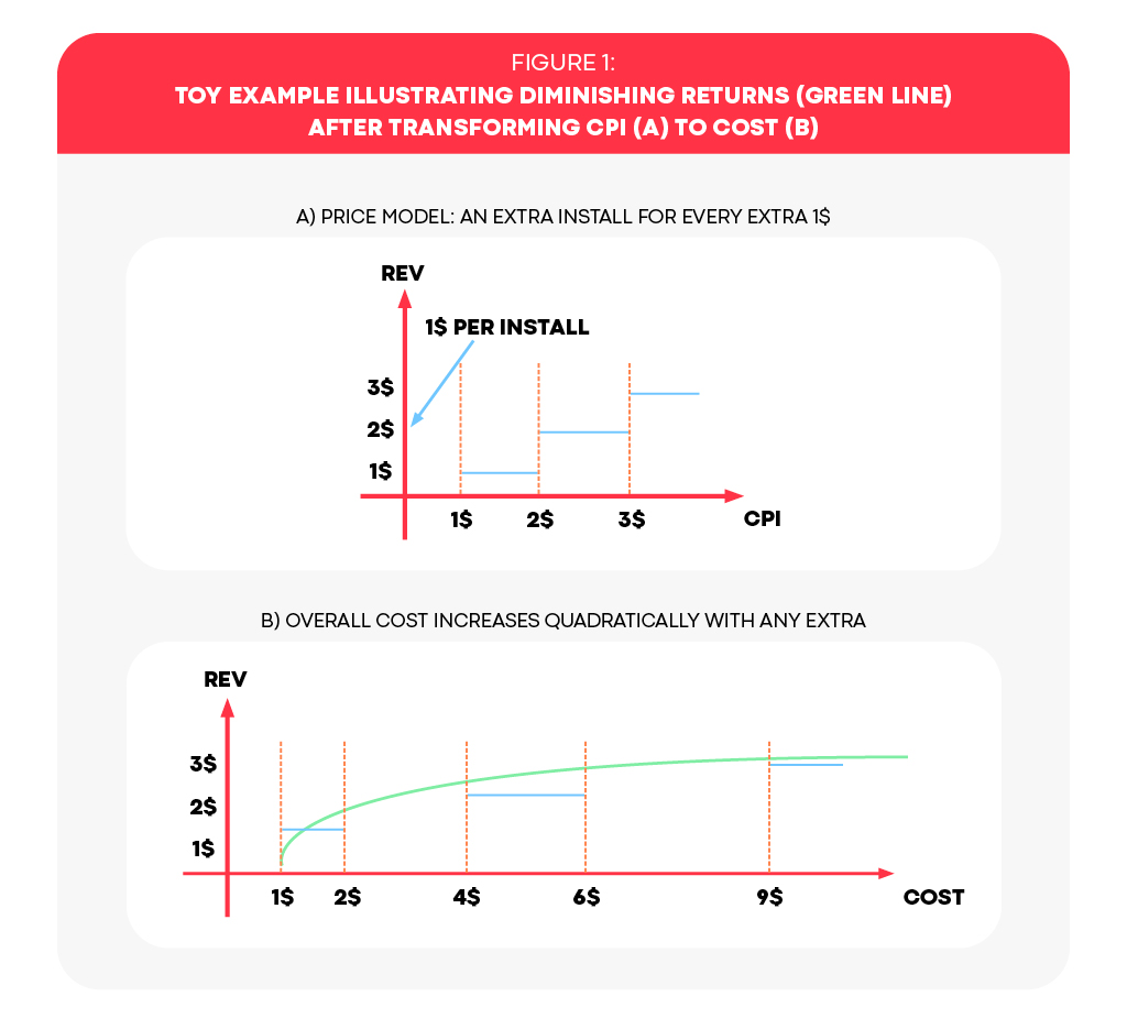
4. Diminishing Returns – Our third law encompasses a well-known economic principle. It states that in order to generate the next dollar of revenue, one must spend at an ever-increasing pace. To illustrate this concept, let’s consider the scenario as in Figure 1, where each acquired user generates revenue of 1$. Suppose our campaign follows a cost-per-install (CPI) model, which means we bid a certain amount per install and, in return, receive a group of users from the media source based on our bid. Since there is no incentive to pay more and receive fewer users, let’s assume that the group size increases as our bid increases. For simplicity, let’s say that for a bid of \(X\) dollars, we receive \(X\) users. Therefore, our total revenue is \(X\) dollars. However, our cost is actually \(X\) squared (\(X^2\)). In other words, to generate a revenue of 1 dollar, we only had to pay 1 dollar. However, to increase the revenue to 2 dollars, we would need to pay 4 dollars, an additional 3 dollars. Similarly, to achieve 3 dollars in revenue, we would need to pay 9 dollars, an additional 6 dollars. Mathematically, our cost-to-revenue (KPI) function should be monotonic increasing to justify the increase in cost and concave to reflect the diminishing returns as the cost increases.

The Analytic String Model

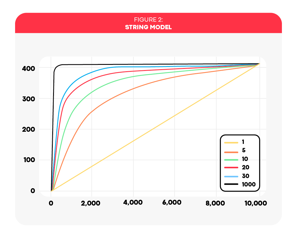
In conclusion, our model is a one-dimensional function, which is both increasing and concave, with two anchors: the origin and the couple \(<cost, KPI>\) of the respective average time frame. This realization promotes the search for a family of functions parameterized by a single parameter, which somehow control our function’s rate of increment. We call it a string model due to its appearance as a string, with ends pinned to the two anchors (see Figure 2).

The mathematical properties are achieved using trigonometric functions:

\(f(x)=tan^{-1} \left( \theta \cdot tan \left( \frac{\pi x}{2 \Delta} \right) \right)\)

Note that \(\Delta\) is a fixed scale factor that represents some upper bound on \(x\). This is required, as \(tan\) is a periodic function, and may return negative values once its argument evaluates a value exceeding \(\pi /2\).

In such a case, our KPI model becomes:

\(r_i^k(c_i)=R \cdot \frac{f(c_i)}{f(C)}\)

Where \(C\) and \(R\) are the cost and KPI dictated by the time-invariance law and. It’s now apparent that the scale factor \(\Delta\) should be no lower than the minimum – between our local constraint, \(B_i^H\), and the maximum cost recorded in our dataset.

The main benefit of the string model is its flexibility in capturing any curvature using \(\theta\), going from a linear line (\(\theta=1\)) all the way to a step function (\(\theta \rightarrow \infty\)), and it varies smoothly with increasing \(\theta\).

Revisiting the Dataset

Let’s consider our dataset, which comprises pairs of (cost, KPI) recorded over cohorts. Given that each cohort consists of only a few tens of users, and considering the sparsity issue of our user data, it is unlikely that the scatterplot of our cohort points would exhibit a clear monotonic increasing and concave relationship between cost and the KPI. While our model has only a single parameter, fitting the data may not pose a challenge. However, it becomes difficult to interpret the quality of the fit when dealing with noisy data.

Instead, we aim to adopt a different perspective on our data, one that would generate a scatterplot that adheres to the diminishing returns law. In other words, we seek an algorithmic approach to systematically transform our original dataset into a new one with the desired properties. To do so, let’s engage in a thought experiment:

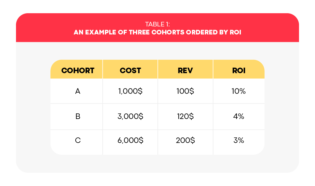
Imagine you’ve just closed a month of acquisition, spending 10K$ with a return of 420$ in total. More specifically, assume that you’ve acquired three cohorts,  and , with the cost and revenue listed in Table 1. Imagine that you’re given the chance to go back in time and buy only the best cohort, , where “best” is in terms of return-on-investment (ROI). Despite the improvement in ROI, the overall spending has decreased to 10% of the original budget, so you’re asked to augment your acquisition by one more cohort. In this scenario, the best choice is cohort B, as it is the best available option after having already acquired cohort A. This selection ensures that the overall ROI remains maximized when considering the acquisition of two cohorts from last month’s inventory. Consequently, the ROI decreases to 5.5%, but our spending increases to 40% of the original budget. Finally, if this increase in spending is still insufficient, we are compelled to revert to our original performance and acquire all three cohorts, thereby utilizing the entire initial budget and reducing the ROI to its original value. Therefore, the three original cohorts serve as a basis for three purchase plans, each is optimal in ROI per the quantity of cohorts we must pick again from the last month’s inventory.

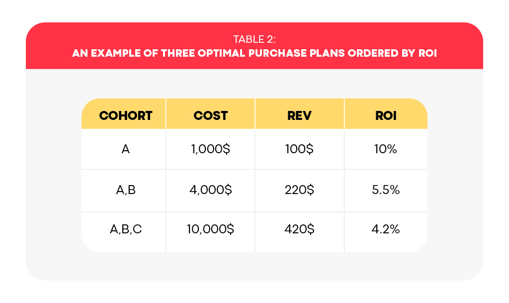
What did we accomplish in this thought experiment? Firstly, we transitioned from considering the cost of individual cohorts to examining the cumulative cost over multiple cohorts. Secondly, we rearranged the order of the cohorts based on their decreasing return on investment (ROI). However, these two steps pose certain unrealistic expectations, even if the upcoming month featured the exact same cohort inventory:

First, if our conclusion is to decrease costs, it implies that we should spend until we reach our target cost and then cease spending for the remainder of the month. However, this approach is unrealistic, since media sources expect daily spending over the entire month. Decreasing the average daily spend may introduce nonlinear effects that significantly alter the behavior of cohorts.

Secondly, we must acknowledge that we have no control over the order in which cohorts are acquired. Therefore, the cost-to-KPI curve can be considered as an upper bound. Nevertheless, if we allocate sufficient resources to acquire a substantial number of users, we can invoke a notion of typicality, similar to the scenario of tossing a coin where heads and tails occur in roughly equal proportions over a long sequence of tosses.

Moreover, budget allocation is a relative problem. Even if the upper bound is not precisely defined, we can still rank the business units (BUs) appropriately since they all possess a similar advantage.

It’s worthwhile to note that the dataset transformation algorithm mentioned above can be seen as the optimal solution to a continuous variant of the Knapsack Problem (Figure 3). In this context, we are presented with a collection of items, each having a weight and a corresponding value. The objective is to maximize the total value of the items we select to include in our bag, while ensuring that the sum of their weights does not exceed the bag’s carrying capacity.

The continuous variant treats the decision variables as continuous, meaning that we have the flexibility to “break” an item and only include a portion of its value and weight proportional to our needs. This variant allows for an efficient greedy algorithm: we simply sort the items in descending order based on their relative value-to-weight ratio, and then select them one-by-one until reaching an item that would violate the weight constraint. We then take only the proportion of that last item needed to completely fill the bag to its capacity

Basically, our thought experiment described a collection of continuous Knapsack Problems, with capacity matching the total cost (weight) of the “best” cohorts (items). Therefore, there was no need to “break” any cohort into partial values or weights. At first, considering only the original cohort acquisitions may seem quite limiting, as in our example above. Nevertheless, this is exactly where our analytical String model supplements, serving as a method that allows to both interpolate and extrapolate the data, as well as allow the optimizer to imply new budgets to explore.

Back to the Optimization Program

Now that \(r_i^k\) has been well defined, we can explore the method to solve the optimization program. Although our functions are concave and the global constraint is linear, facilitating the use of some convex optimization engine, we opt for a different approach using mixed-integer programming (MIP). This choice is driven by the recognition that the budget offered to the media source by the advertiser is often a nominal figure, subject to potential variations when it comes time to make the actual payment. This randomness stems from the inherent unpredictability in the media buying world, where media sources cannot guarantee the exact volume of users they will provide.

For instance, in cost-per-install (CPI) campaigns, the payment event occurs only when a user decides to install the advertised product, which can happen several days after the initial ad impression. To avoid wasting time, media sources may generate multiple impressions concurrently, anticipating that only a fraction of them will result in installations. As a result, the media source will continue displaying our ad as long as there is remaining budget and will only cease when it detects that the budget has been depleted. Therefore, the media source will continue to show impressions of our ad as long as there is some budget left and stop only once it detects that the budget has been exhausted.

However, beyond this limit, new installations may still occur, leading to an increase in the overall cost beyond the nominal budget.

By using a MIP solver, we may limit the selected cost to a multiple of some reasonable figure, such as 1000$. Additionally, the MIP solver can provide information on whether it has converged to the global optimal solution, offering a certificate of success. To handle the non-linear concave function, we relax it into a piecewise linear function using special-ordered-sets.

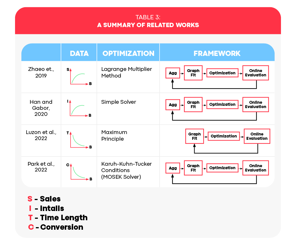
Related works

Budget allocation has garnered attention by academics and industry professionals (Zhao et al., 2019; Han and Gabor, 2020; Luzon et al., 2022; and Park et al., 2022). In Table 3, we summarize prior works on data representation,

Conclusion

In this blog, we introduced a streamlined computational framework for optimizing budget allocation. Our approach focuses on the key metrics at the extremities of the acquisition process: the cost input and the KPI output. This framework enables us to model various business units, whether it is a single campaign or an entire media source hosting multiple campaigns, while remaining adaptable to different tiers of business units and media buying methods. By employing the String Model with a Knapsack-style reshuffle of our data, we achieve consistent and economically sensible modeling of business units. Furthermore, the use of the MIP solver provides a guarantee of optimality in our solutions, as well as control over the allocated nominal budgets’ resolution.

Tags