Multi-Dimensional Classification and the Importance of Correlations
By Yotam Rotholz
Multi-Dimensional Classification (MDC) algorithms can lead to significantly improved results in classification problems with correlated labels, as we have discovered through our own experience solving such a task. In this post, we will share what we’ve learned. The post will begin with the basics of what MDC is and will then proceed to a discussion of various relevant algorithms. An in-depth explanation of the Ensemble of Classifier Chains algorithm will also be provided. In the second post of the series, we will demonstrate examples of MDC performance using our data.

Introduction
In supervised learning, most classification models predict a single output that corresponds to the category, or class, that the input objects may belong to. For example, a neural network model can learn to classify emails (the input objects) as either spam or not spam (the output). However, in many real-world applications, the tasks are more complex as objects are described or classified along multiple dimensions. Each dimension represents a different category; for example, a vehicle could be simultaneously classified by its type (car, bus, or truck), color (white, red, or gray), and brand (Mercedes, Subaru, or Ford).
An approach to tackle multi-dimensional tasks is to consider a classifier for each dimension. For example, in the vehicle example, we could use three models: one for its type, one for its color, and one for its brand. Another approach would be to use a single model that predicts the cartesian product of the three dimensions (e.g., car-white-Mercedes, car-white-Subaru). However, what happens when there are correlations between the output dimensions, such as Subaru not tending to produce red cars or Mercedes is the only truck manufacturer?
The first approach mentioned ignores such correlations altogether, while the second approach implicitly ‘covers’ these correlations in a highly inefficient manner by considering all possible combinations of labels, even non-existing ones. Consequently, these approaches may result in lower performance and poor computational efficiency. To address this, we can incorporate dependencies among the output dimensions appropriately and improve our results by using the Multi-Dimensional Classification (MDC) framework.
MDC solves classification tasks along various dimensions simultaneously [1]. It offers a variety of algorithms that optimize overall prediction performance by exploiting correlations between target variables, leading to typical 5-10% uplifts in performance (in our task, we saw even higher uplifts). In this post, we begin by providing useful information about MDC and how it differs from other classification approaches. We will then discuss a few naïve and advanced MDC algorithms and focus on the Ensemble of Classifier Chains (ECC) [2].
This algorithm is relatively easy to learn for those new to the topic, is frequently used as a benchmark, and encompasses many of the ideas of more advanced and modern approaches.
What is Multi-Dimensional Classification?
To understand MDC let us differentiate it first from other classification types. The first one will be the binary classification task, which includes a single output variable that has only two possible values (as shown in Figure 1, top row). An example of this classification type is classifying whether an email is spam or not.
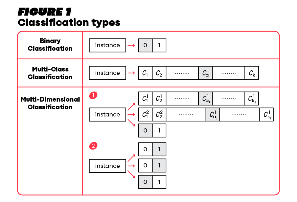
Then, if there are three or more possible output values, it is a Multi-Class Classification task (as shown in the second row). Continuing with the spam classification example, Multi-Class Classification is a system that can classify an email as spam, important, social, etc.
Now, MDC (as shown in the bottom row) represents the scenario where an instance may have several outputs, each corresponding to a different dimension of the instance. To Illustrate MDC, consider the case where an autonomous car is trained to classify its surrounding vehicles according to their type, brand, and color (just as in the vehicle example above). MDC may involve binary class spaces together with multi-class class spaces, as depicted by index 1 at the bottom row. A simpler variant of MDC is Multi-Label Classification, where each of the labels has a binary class space (bottom row index 2). For example, a photo may include multiple classes in the scene, such as a bicycle‘, ‘a traffic light‘, and ‘a person, and the model learns to predict the occurrence of each class (for example, is there a bicycle in this photo? Yes or no? Is there a person? Yes or no? etc.)
It’s worth mentioning that Multi-Label Classification is a variant of MDC, and solutions that have been used to solve multi-label problems have been applied to multi-dimensional ones.
Basic modeling approaches
To demonstrate a couple of basic approaches for Multi-Label Classification, let’s consider an observation with a set of features that are mapped to three binary labels, the class variables (Figure 2).
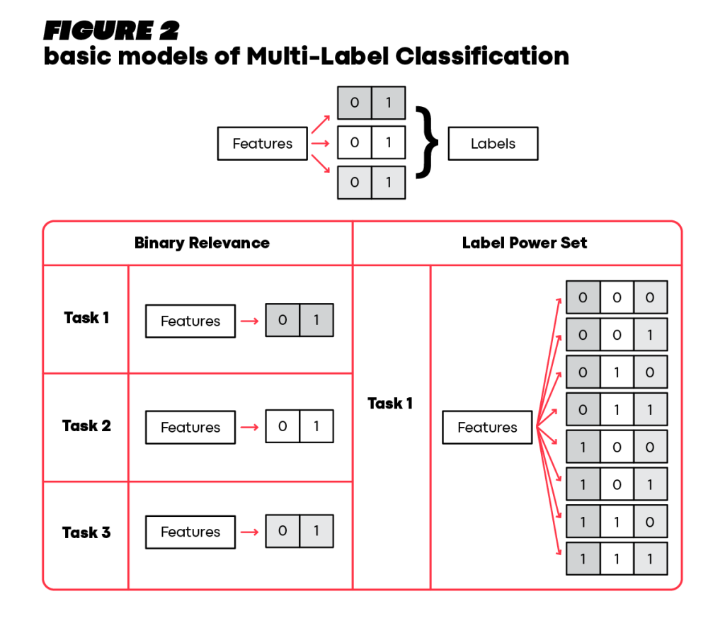
In Binary Relevance, the problem of Multi-Label Classification is decomposed into three separate tasks. For each task, a base model, such as logistic regression, SVM, or decision trees, is trained for the relevant binary label [1]. During inference, the output is a set of three values corresponding to each class variable. By contrast, the Label Power Set approach transforms the 3 binary class variables into a single class space with eight possible values, one for each combination, by creating a cartesian product of the class spaces and subsequently solving the problem as a single classification task [1].
Both the Binary Relevance and Label Power Set approaches are commonly used for solving Multi-Label Classification problems because they are simple to comprehend and implement. However, they are considered naïve approaches because they do not incorporate label correlations appropriately. The Binary Relevance approach does not take into account such dependencies at all, as it trains independent base models. The Label Power Set approach incorporates such correlations but in an extremely inefficient manner. While all possible combinations of the class spaces are considered, close combinations, such as those that share the same values in all class spaces except for one, are treated as equally distant from each other. Additionally, considering all possible combinations, even non-existing ones, can lead to extreme sparsity and become computationally expensive.
A more advanced algorithm for solving MDC problems combines the Binary Relevance and Label Power Set approaches while incorporating label dependencies effectively. This algorithm maps conditional dependencies among the class variables and partitions them into groups called “super-classes.” In this scenario, a super-class can stem from a single class variable or several class variables, depending on the dataset. For each super-class, the cartesian product of its class variables serves as a “single class variable” to a dedicated base model. For example, if we have three class variables \(\{Y_{1}, Y_{2}, Y_{3}\}\), and \(Y_{1}\) and \(Y_{2}\) are dependent but \(Y_{3}\) is independent of \(Y_{1}, Y_{2}\), then the partitions would be \(\theta = \{(Y_{1}, Y_{2}), (Y_{3})\}\). This case is then solved by two base models, one for the cartesian product of \((Y_{1}, Y_{2})\) and a second for \(Y_{3}\). This approach, therefore, harnesses the Label Power Set within partitions and the Binary Relevance between different partitions, making it more efficient than just considering the Label Power Set alone [3].
Ensemble of Classifier Chains
The Ensemble of Classifier Chains (ECC) is one of the most popular algorithms in the field of MDC. It combines simplicity and training efficiency, while also exploiting inter-class correlations. Its flexibility in terms of its different hyper-parameters, and its relatively high-quality performance, have made it one of the main benchmarks for innovative algorithms [3]. These reasons led us to use this algorithm in our own research and to discuss it more thoroughly in this post.
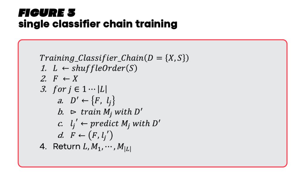
A classifier chain represents a sequence of base models, each of which is dedicated to predicting a certain class space. The process of training a single classifier chain is described in Figure 3. Training is done on a dataset \(D\) that is composed of explanatory variables \((X)\) and class variables \((S)\). First, the order of the class variables is randomly shuffled. The current feature space \((F)\) is initialized to be the original feature space \((X)\). Then, the algorithm iterates through the shuffled order of class variables and trains base models sequentially (rows 3a-d in Figure 3). At iteration \(j\), model \(M_{j}\) is trained to predict class variable \(l_{j}\) using feature space \(F\). The first base model, \(M_{1}\), that predicts first class variable (\(l_{1}\)), is effectively trained with the original feature space (i.e. \(X\)). Then, the predictions of the trained model (\({l_{1}}^{‘}\)) are appended to \(F\), enriching it for the next base models to train. \(M_{2}\) is trained with the augmented feature set, where \({l_{1}}^{‘}\) serves as an additional feature to \(X\). This process continues until all base models for all class variables are trained.
Data augmentation is a very popular technique in MDC problems and will be further demonstrated in the next blog post.
The inference flow of a single classifier chain is quite similar to the training flow, i.e., gradual inference along the class variables in the order that was set during the training phase. Eventually, each classifier chain provides a set of predictions – one prediction per class space [2]. Rather than having a single classifier chain, the ECC algorithm constructs multiple uncorrelated classifier chains. An ensemble of many classifier chains is expected to generalize better and thus outperform an ensemble of few classifier chains.
How are uncorrelated classifier chains generated? Answer: Randomization, Randomization, Randomization.
- Random order of class variables – this point was covered earlier.
- A random subset of rows – samples vary among classifier chains.
- A random subset of columns – different subsets of features are utilized for each classifier chain.
Figure 4 illustrates how the ECC training is done.
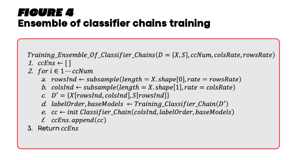
The function signature demonstrates some of the potential hyperparameters for this algorithm:
- \(ccNum\) – number of classifier chains to train.
- \(colsRate\) – the rate of columns to keep. The range is between 0 and 1, where 1 indicates keeping all columns.
- \(rowsRate\) – the rate of rows to keep. The range is between 0 and 1, where 1 indicates keeping all observations.
The parameters \(colsRate\) and \(rowsRate\) define the portion of data that should be used for training. What is the incentive to use a subset of data when training a classifier chain? There are several reasons.
First, since some base models may converge slowly until reaching optimized parameters, reducing the dataset size could facilitate convergence.
Second, to gain model generalization, chain classifiers are expected to yield different predictions. However, this is not always the case. Analytical base models (like SVM) converge to the same model given a certain dataset.
Let’s look at the following settings:
- Class spaces amount: 2.
- Base model: SVM.
- \(ccNum\): 3.
- \(colsRate\): 1.
- \(rowsRate\): 1.
Given the fact that there are two class spaces and three classifier chains, a certain order will surely repeat, because two class spaces have two distinct orders (1->2, 2->1). Equal datasets train the classifier chains when subsample rates are 1. All of the above leads to the case that at least 2 out of 3 classifier chains end up with the same trained base models and yield identical predictions.
Eventually, subsampling is not necessary but beneficial in some cases. [2] found that subsampling saves enormous convergence time with slightly degraded prediction performance. Furthermore, the technique of using random subsets to train uncorrelated predictors is quite useful in training machine learning models. This technique is called Bagging and it is the core idea behind the famous Random Forest model.
After covering the algorithm training, the last thing to discuss is algorithm inference. At the inference phase, the predictions of all classifier chains are aggregated into a single prediction per class space. In their research [2], the authors utilized majority vote as an aggregation method for the ensemble predictions, though other aggregation methods could be considered.
Conclusions
We hope that we have managed to convince you to seriously consider using the Multi-Dimensional Classification framework if your classification problem includes several heterogeneous class variables. In this post, we provided information about the theoretical utilization of the Multi-Dimensional Classification approach, a few benchmarks, and a detailed explanation of the Ensemble of Classifier Chains algorithm.
Although this algorithm exploits label dependencies, it offers simplicity, and interpretability and enables convenient hyperparameter tuning. Moreover, it can be trained on top of any base model one chooses, like SVM, Neural Networks, Random Forest, or Catboost.
We hope that the next time you face a Multi-Dimensional Classification problem, you will use an algorithm that considers label correlations, as it would likely end with improved prediction performance.
In the next post, we will present the results of the Ensemble of Classifier Chains on our data. We observed an uplift of more than 10% in prediction accuracy compared to the benchmarks.
References:
- Jia, B. B., & Zhang, M. L. (2021). Maximum margin multi-dimensional classification. IEEE Transactions on Neural Networks and Learning Systems.
- Read, J., Pfahringer, B., Holmes, G., & Frank, E. (2011). Classifier chains for multi-label classification. Machine learning, 85(3), 333-359.
- Read, J., Bielza, C., & Larrañaga, P. (2013). Multi-dimensional classification with super-classes. IEEE Transactions on Knowledge and data engineering, 26(7), 1720-1733.